The curse of multidimensionality.

I wonder how I could possibly navigate a forest full of trails, each with signs promising to take me to the perfect place: the mountain cabin, the secret beach, or that clearing where the sunlight always shines. Fascinated, I might decide to take all the paths at once, juggling between opposite directions.

The result? I’d be left spinning in circles, trapped between possibilities, getting nowhere. Sound frustrating? Well, this is exactly what happens when statistical models try to encompass too many variables at once.

In statistics, this phenomenon is known as the curse of dimensionality. When there are almost as many, or even more, paths (variables) than places to go (observations), classic techniques like regression get caught. The model fits the available data so well that it seems perfect, but in reality it has completely lost its way: it can’t predict anything useful beyond the forest where it was created. It’s as if those paths only exist on a hand-drawn map by a cartographer with too much imagination.

If you continue reading, in this post we will explore how the excess of variables turn models into dead-end labyrinths, where neither R² nor least squares errors can help us escape. If you have ever felt lost among numbers that promised magical solutions, this is your opportunity to learn how to avoid the traps of overfitting.

Let’s try to discern how not to lose our way in the forest of data.

New technologies are to blame

Until not long ago, it was common in biomedicine to handle data sets with quite a number of observations, but with a not very high number of variables in each observation. If we call “n” the number of observations and “p” the number of variables, p used to be much smaller than n.

In this context, most statistical techniques have been designed to work well in this low-dimensional environment, as is the case, for example, with linear regression, the technique we are going to focus on today.

But progress is unforgiving and, over the last two decades, new technologies have radically changed the way we obtain and process information in numerous fields, including biomedicine. Thus, it is not at all unusual to have data sets in which the number of variables (p) is large, while the number of observations (n) is smaller, either due to economic costs or the difficulty of obtaining the data.

Three decades ago we could try to predict life expectancy by looking at the relationship between weight, blood sugar and blood pressure, for example (n = 1000, p = 3). In contrast, today we may be interested in studying the relationship with tens or hundreds of thousands of DNA mutations (so-called polymorphisms, SNPs), to give another typical example (n = 150, p = 3000).

These data sets have become wider than they are long, or, to put it elegantly, they are characterized by high dimensionality.

One might think that this is great, you know, more is better. Surely with more variables we can detect more patterns and associations. But it is not that simple, since the control methods of classical statistical tests may not work very well in high dimensionality contexts and generate totally useless predictive models.

The linear regression example

We saw in a previous post how the least squares method is used to calculate the optimal value of the coefficients of a linear regression model. You can review the topic if you don’t remember it well.

The problem with least squares is that when p approaches, or exceeds, the value of n, this method stops working so well and, even if there is no real relationship between the data, it will estimate coefficient values ​​that will provide a perfect fit to the available data.

Those of you who are more attentive will have already realized that what the model does is overfit the data, which has the disastrous consequence that it cannot be generalized to new data. Think about it, models are created to make predictions with new, unknown data (the ones we use to create them are already known).

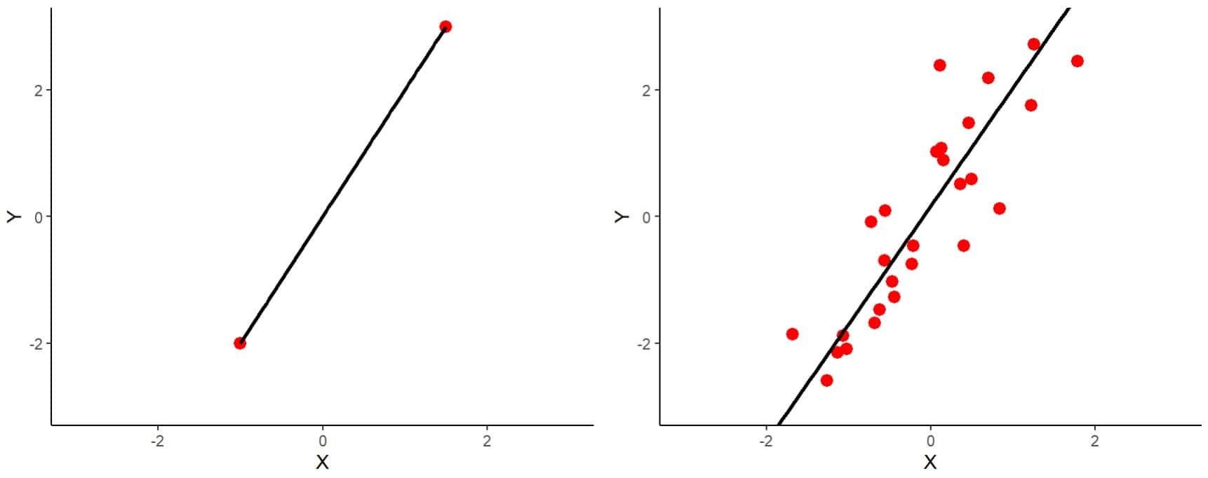
To understand this in an intuitive way, I show you the two graphs in the first figure.

On the left you can see the simplest case of the situation in which n = p represented. We have two variables and two observations. You can see that the regression line fits perfectly, passing through the two observations.

On the right you have a similar example, but with 30 observations (n ​​= 30, p = 2). It is clear that the line cannot pass through all the points as well as it did in the other example. The least squares method is responsible for calculating the coefficients of the model so that the line passes as close as possible to all the points, minimizing the squares of the distances from the points to the line.

It might seem that the first model is better, but let’s think about what will happen when we have a new observation. In fact, the model on the right will be more likely to fit better, with a higher n/p ratio. Well, the same thing happens with a larger number of observations and variables. We are faced with the curse of dimensionality.

In conclusion, when the number of variables approaches or exceeds the number of observations, the least squares equation is too flexible and overfitting occurs.

But it doesn’t end there. The parameters that we normally use to assess the goodness of the model, such as the mean error of the estimates or the coefficient of determination, do not work well either.

The curse of multidimensionality

To show you the latter, we are going to use a fictitious example that I have invented on the fly using the R program. The more adventurous can download the complete script at this link.

To force the situation a little, not too much, I have simulated a data set with 100 observations and 100 variables (n = p = 100). As usual, I have been a bit tricky and only 10 variables have a linear relationship with the target variable. The other 90 variables are pure random noise.

Once created, I divide the data into two subsets, one for training (70 observations) to create the models and one for testing (30 observations) to test them. Logically, in these two subsets the number of variables exceeds the number of observations (n ​​< p).

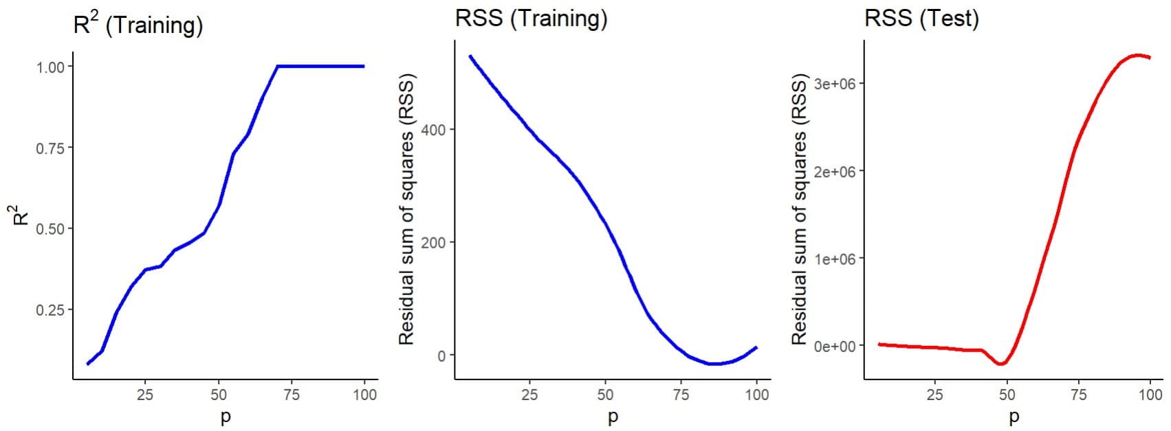
Finally, I have assembled consecutive models with an increasing number of predictive variables, starting with five and adding five more in each consecutive model. For all of them I have calculated the coefficient of determination (R²), as an indicator of the model’s performance, and the sum of the squares of the residuals (SSR), as an indicator of the error, as you can see in the second figure.

Let’s first look at the blue graphs, which represent the two parameters obtained when building the models with the training data. We see how the R² increases progressively as we add more predictive variables to the model, so that it reaches a value of 1 when we include about 70 variables or more.

Something similar happens with the model’s errors (the SSR), which decrease until they reach almost zero, more or less at the same point where R² approaches 1.

This might seem great to us. If R² represents the percentage of the variance of the data that is explained by the model, a value of 1 would tell us that the model is perfect, since it captures practically all the variance of the data, with an error that is practically negligible.

What is the problem? Let’s now look at the graph with the red line, made by testing the models with the test data, not used for the actual development of the model. We can see how the error of the model when making predictions shoots up from a certain number of variables, in this case about 50 variables.

The interpretation is simple. Putting so many variables in a model, most of them unrelated to the variable we want to predict, causes an overfitting of the model to the training data, but a calamitous lack of capacity to generalize the predictions when we present it with new data.

The lesson to be learned is that we have to very carefully evaluate the results with data sets with a large number of variables and never, ever forget to check the performance of the model on an independent data set.

As in many other aspects of life, more is not always better and quality may be more important than quantity, which leads us to think about the possible solution to this problem.

The solution to the problem

The solution to the problem of high dimensionality is clear: to reduce dimensionality, for which we have numerous possibilities.

The simplest would be to make a selection of variables with the most traditional methods, such as forward stepwise selection. We could also use regularization techniques such as lasso regression, which allows us to reduce the number of variables.

Finally, we can apply dimensionality reduction techniques using principal component analysis or other types of machine learning algorithms, such as decision trees, to select a reduced number of variables that includes those that are truly important for building the model.

We’re leaving…

And here we will leave it for today.

We have seen one of the effects of the so-called curse of dimensionality. Contrary to what one might think, greatly increasing the number of predictor variables in a model can be counterproductive when creating a model that must have some predictive capacity.

The variables must be carefully selected, particularly when there are many in relation to the number of observations, and only those that can really influence its predictive capacity must be included in the model. The rest of the variables will only add noise and contribute to the risk of overfitting. As always, a balance must be sought between the ability to fit (the bias of the model) and the ability to generalize (the variance of the model).

Of course, this is often easier said than done. It may happen that some of the predictor variables are related to each other, that is, we can face the problem of multicollinearity. In these cases, some variables may be described as linear combinations of other variables, which will make it difficult to find out which ones are really important for the model and will prevent us from estimating the best values ​​for the regression coefficients. But that is another story…