Chi-square homogeneity test.

The chi-square homogeneity test compares proportions from various samples to see if they come from the same population.
There’s nothing more unfortunate that being a black sheep. We know that the term is commonly used to refer to someone who stands out in a group or a family, usually due to a negative trait. But black sheep, in the literal sense of the word, exist in the real world. And as their wool is less valued than that of white sheep, it is easy to understand the shepherd’s annoyance when he discovers a black sheep in his flock.
So, we, to compensate for some discrimination against black sheep, will count sheep, but only black. Let’s suppose that during a hallucinatory attack we decide that we want to become shepherds. We go to a cattle fair and look for a herd to buy it.
Counting sheeps
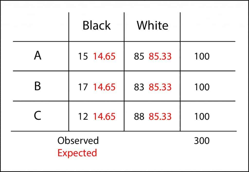
But then, as we are rookies on the business, they’ll try to sell us the herds that have more black sheep. So, we take three random samples of 100 sheep from three herds, A, B and C, and count the number of black sheep: 15, 17 and 12. Does this mean that flock C is the one with less black sheep?. We cannot be sure with these data alone.
We may have, just by chance, selected a sample with less black sheep when, actually, this is the flock with more of them. As the differences are small, we may venture to think that there’re not great differences among the three herds and that the observed ones are simply due to random sampling error. This will be our null hypothesis: the three herds are similar in proportion of black sheep. We can now make our hypothesis testing.
We know that we can use the analysis of variance to compare means of different populations. This test is based on whether the differences among groups are greater than differences due to random sampling error. However, in our example, we have no means, but percentages. How can we do the hypothesis contrast?. When we want to compare counts or percentages we have to resort to the chi-square test, although the reasoning is very similar: to check if differences among expected and observed values are large enough.

Chi-square homogeneity test
Once we have calculated observed and expected values, we calculate the differences among them. If we sum up them now, positive differences would cancel out negative ones, so we squared them before, as we do to calculate the standard deviation of a data distribution.
Finally, we must standardize these differences dividing them by their expected values. It is not the same to expect one and to observe two than to expect 10 and to observe 11, although difference in both cases is equal to one. And once we have all these standardized residuals we just have to add them to obtain a value that someone dubbed as Pearson’s statistic, also known as λ.
If you do the calculation you’ll see that λ = 1.01. And that’s a lot or a little?. It so happen that λ approximately follows a chi-square probability distribution with, in our case, two degrees of freedom (rows-1 by columns-1), so we can calculate the probability to get a value of 1.01. This value is the p-value, which is 0.60. As it is greater than 0.05, we cannot reject our null hypothesis and we have to conclude that there’s not statistically significant differences among the three herds. I’d buy the cheapest of them.
These calculations can be easily done with a simple calculator, but it is usually faster to use any statistical software, especially when dealing with large contingency tables, with larger numbers or with figures with many decimal numbers.
We’re leaving…
And here we stop counting sheep. We have seen the usefulness of chi-square test to check homogeneity of populations, but chi-square is use for more things, like for testing the goodness of fit of two populations or the independence of two variables. But that’s another story…
