Diagnostic screening.

The characteristics of the diagnostic screening and the ways of calculating the prevalence of the disease from its results are described.
Nobody is perfect. It is a fact. And a relief too. Because the problem is not to be imperfect, it is inevitable. The real problem is to believe one being perfect, to be ignorant of one’s limitations. And the same goes for many other things, such as diagnostic tests used in medicine.
But this is a real crime with diagnostic tools because, beyond its imperfection, it is possible to misclassify healthy and sick people. Don’t you believe me?. Let’s make some reflections.
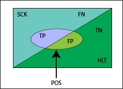
To begin with, take a look at the Venn’s diagram I have drawn. What childhood memories these diagrams bring to me!. The filled square symbolizes our population in question. Up the diagonal are the sick (SCK) and down it the healthy (HLT), so that each area represents the probability of being SCK or HLT.
The area of the square, obviously, equals 1: we can be certain that anybody will be healthy or sick, two mutually excluding situations. The ellipse encompasses the subjects undergoing the diagnostic test and getting a positive result (POS). In a perfect world, the entire ellipse would be above the diagonal, but in the real imperfect world the ellipse is crossed by the diagonal, so the results can be true POS (TP) or false (FP), the latter when are obtained in healthy. The area outside the ellipse would be the negatives (NEG), which, as you can see, are also divided into true and false (TN, FN).
Screening performance
Now let’s transfer this to the typical contingency table to define the probabilities of different options and think about a situation where we still have not carried out the test. In this case, the columns condition the probabilities of the events of the rows. For example, the upper left box represents the probability of POS in the SCK (once you are sick, how likely you are to get a positive result?), which we call the sensitivity (SEN).
For its part, the lower right represents the probability of a NEG in a HLT, which we call specificity (SPE). The total of the first column represents the probability of being sick, which is nothing more than the prevalence (PRV), and so we can discern what the significance of the probability of each cell is. This table provides two features of the test, SEN and SPE, which, as we know, are intrinsic characteristics of the test whenever it is performed under similar conditions, even though if the populations are different.

And what about the contingency table once you have carried out the test?. A subtle, but very important, change has taken place: now the rows condition the probabilities of the events of the columns. The total of the table do not change but do look now at the first cell, that represents the probability of being SCK given that the result has been POS (when positive, what is the probability of being sick?). And this is no longer the SEN, but the positive predictive value (PPV). The same applies to the lower right cell, which now represents the probability of being HLT given that the result has been NEG: the negative predictive value (NPV).
So we see that before performing the test we can usually will know its SEN and SPE, while once perform the test we can calculate its positive and negative predictive values, remaining these four test’s characteristics linked through the magic of Bayes’ theorem. Of course, regarding PPV and NPV there’s a fifth element to take into account: the prevalence. We know that predictive values vary depending on the PRV of the disease in the population, while SEN and SPE remain unchanged.

An example of screening
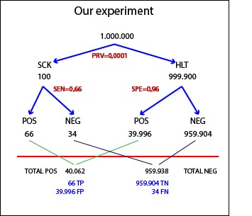
And all this has its practical expression. Let’s invent an example to messing around a bit more. Suppose we have a population of one million inhabitants in which we conduct a screening for fildulastrosis. We know from previous studies that the test SEN is 0.66 and SPE is 0.96, and the prevalence of fildulastrosis is 0.0001 (1 in 10,000); a rare disease that I would advise you not to bother to look for it, if anyone has thought about it.
Knowing the PRV is easy to calculate that in our country there are 100 SCK. Of these, 66 will be POS (SEN = 0.66) and 34 will be NEG. Moreover, there will be 990,900 healthy, of which 96% (959904) will be NEG (SPE = 0.96) and the rest (39,996) will be POS. In short, we’ll get 40,062 POS, of which 39,996 will be FP. No one feel scared about the high number of false positives.
This is because we have chosen a very rare disease, so there are many FP even though the SPE is quite high. Consider that in real life, we’d need to do the confirmatory test to all these subjects to finish confirming the diagnosis only in 66 people. Therefore, it’s very important to think well if the screening is worth doing before starting to look for the disease in the population. For this and many other reasons.
We can now calculate the predictive values. PPV is the ratio between true and the total of POS: 66/40062 = 0.0016. So, there will be one sick in 1,500 positive, more or less. Similarly, the NPV is the ratio between true and the total of NEG: 959904/959938 = 0.99. As expected, given the high SPE of the test, to get a negative result makes it highly improbable to be sick.
What do you think? Is it a useful test for mass screening with such a number of false positives and a PPV of 0.0016?. Well, while it may seem counterintuitive, if we think about it for a moment, it’s not so bad. The pretest probability of being SCK is 0.0001 (PRV). The posttest probability is 0.0016 (PPV). So, their ratio has a value of 0.0016/0.0001 = 16, which means we have multiplied by 16 our ability to detect the sick. Therefore, the test doesn’t seem so bad, but we must take into account many other factors before starting to screen.
Screening calculations
All this we have seen so far has an additional practical application. Suppose you only know SEN and SPE, but we don’t know the PRV of the disease in the population that we have screened. Can we be estimated it from the results of the screening?. The answer is, of course, yes.
Imagine again our population of one million subjects. We do the test and get 40,062 positive. The problem here is that some of these (the most) are FP. Also, we don’t know how many patients have tested negative (FN). How can we get then the number of sick people?. Let’s think about it for a while.
We have said that the number of patients will be equal to the number of POS minus the number of FP and plus the number of FN:
Nº sick = Total POS – Nº FP + Nº FN
We have the number of POS: 40,062. The FP will be those healthy (1-PRV) who get positive being healthy (or the healthy that doesn’t get NEG: 1-SPE). Then, the total number of FP will be:
FP = (1-PRV)(1-SPE) x n (1 million, the population’s size)
Finally, FN will be sick people (PRV) which don’t get a positive (SEN-1). Then, the total number of FN is:
FN = PRV x (1-SEN) x n (1 million, the population’s size)
If we substitute the total of FP and FN in the first equation with the values we’ve just derived, we can get the PRV, obtaining the following formula:

We can now calculate the prevalence in our population:

We’re leaving…
Well, I think one of my lobes has just melted down, so we’ll have to leave it there. Once again, we’ve seen the magic and power of number and how to make that the imperfections of our tools work in our favor. We could even go a step further and calculate the accuracy of the estimate we’ve done. But that’s another story…
