Cohort studies.

The characteristics of cohort studies, their measures of association and impact, and their most characteristic features are described.
What a fellows, those Romans!. They came, they saw and they conquered. With those legions, each one with ten cohorts, each cohort with almost five hundred Romans with their skirts and strappy sandals. The cohorts were groups of soldier that were in reach of the speech of the same boss. They always went forward, never retreating. This is how you can conquer Gaul (though not entirely, as is well known).
Cohort studies characteristics
In epidemiology, a cohort is also a group of people who share something, but instead of being the boss’s harangue it is the exposure to a factor that is studied over time (neither the skirt nor the sandals are essential) .
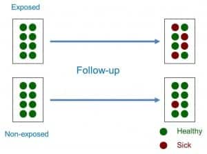
Thus, a cohort study is a type of observational, analytical design, of anterograde directionality and of concurrent or mixed temporality that compares the frequency with which a certain effect occurs (usually a disease) in two different groups (cohorts), one of them exposed to one factor and another not exposed to the same factor (see attached figure).
Therefore, sampling is related to exposure to the factor. Both cohorts are studied over time, which is why most of the cohort studies are prospective or of concurrent temporality (they go forward, like the Roman cohorts). However, it is possible to do retrospective cohort studies once both the exposure and the effect have occurred. In these cases, the researcher identifies the exposure in the past, reconstructs the experience of the cohort over time and attends in the present to the appearance of the effect, which is why they are studies of mixed temporality.
We can also classify the cohort studies according to whether they use an internal or external comparison group. Sometimes we can use two internal cohorts belonging to the same general population, classifying the subjects in one or another cohort according to the level of exposure to the factor. However, other times the exposed cohort will interest us because of its high level of exposure, so we will prefer to select an external cohort of subjects not exposed to make the comparison between both.
Another important aspect when classifying the cohort studies is the time of inclusion of the subjects in the study. When we only select the subjects that meet the inclusion criteria at the beginning of the study, we speak of a fixed cohort, whereas we will speak of an open or dynamic cohort when subjects continue to enter the study throughout the follow-up. This aspect will be important, as we will see later, when calculating the association measures between exposure and effect.
Finally, and as a curiosity, we can also do a study with a single cohort if we want to study the incidence or evolution of a certain disease. Although we can always compare the results with other known data of the general population, this type of designs lacks a comparison group in the strict sense, so it is included within the longitudinal descriptive studies.
When followed up over time, the cohort studies allow us to calculate the incidence of the effect between exposed and not exposed, calculating from them a series of association measures and specific impact measures.
Association measures in cohort studies
In studies with closed cohorts in which the number of participants does not change, the measure of association is the relative risk (RR), which is the ratio between the incidence of exposed (Ie) and unexposed (I0): RR = Ie / I0.
As we know, the RR can value from 0 to infinity. A RR = 1 means that there is no association between exposure and effect. A RR <1 means that exposure is a factor of protection against the effect. Finally, a RR> 1 indicates that exposure is a risk factor, the greater the value of the RR.
The case of studies with open cohorts in which participants can enter and leave during the follow-up is a bit more complex, since instead of incidences we will calculate incidence densities, a term that refers to the number of cases of the effect or disease that they occur referring to the number of people followed by each follow-up time (for example, number of cases per 100 person-years). In these cases, instead of the RR we will calculate the incidence density ratio, which is the quotient of the incidence density in exposed divided by the density in not exposed.
Impact measures in cohort studies
These measures allow us to estimate the strength of the association between the exposure to the factor and the effect, but they do not inform us about the potential impact that exposure has on the health of the population (the effect that eliminating this factor would have on the health of the population). For this, we will have to resort to the measures of attributable risk, which can be absolute or relative.
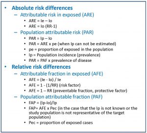
There are two absolute measures of attributable risk. The first is the attributable risk in exposed (ARE), which is the difference between the incidence in exposed and not exposed and represents the amount of incidence that can be attributed to the risk factor in the exposed. The second is the population attributable risk (PAR), which represents the amount of incidence that can be attributed to the risk factor in the general population.

In the attached table you can see the formulas that are used for the calculation of these impact measures.
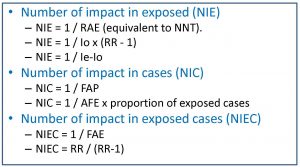
The problem with these impact measures is that they can sometimes be difficult for the clinician to interpret. For this reason, and inspired by the calculation of the number needed to treat (NNT) of clinical trials, a series of measures called impact numbers have been devised, which give us a more direct idea of the effect of the exposure factor on the disease. in study. These impact numbers are the number of impact in exposed (NIE), the number of impact in cases (NIC) and the number of impact in exposed cases (NIEC).
Let’s start with the simplest one. The NIE would be the equivalent of the NNT and would be calculated as the inverse of the absolute risk reduction or of the risk difference between exposed and not exposed. The NNT is the number of people who should be treated to prevent a case compared to the control group. The NIE represents the average number of people who have to be exposed to the risk factor so that a new case of illness occurs compared to the people who are not exposed. For example, a NIE of 10 means that out of every 10 exposed there will be a case of disease attributable to the risk factor studied.
The NIC is the inverse of the PAF, so it defines the average number of sick people among which a case is due to the risk factor. An NIC of 10 means that for every 10 patients in the population, one is attributable to the risk factor under study.
Finally, the NIEC is the inverse of the AFE. It is the average number of patients among which a case is attributable to the risk factor.

As a culmination to the previous three, we could estimate the effect of the exposure on the entire population by calculating the number of impact on the population (NIP), for which we have only to do the inverse of the ARP. Thus, a NIP of 3000 means that for every 3,000 subjects of the population there will be a case of illness due to exposure.
Bias in cohort studies
Another aspect that we must take into account when dealing with cohort studies is their risk of bias. In general, observational studies have a higher risk of bias than experimental studies, as well as being susceptible to the influence of confounding factors and effect modifying variables.
The selection bias must always be considered, since it can compromise the internal and external validity of the study results. The two cohorts should be comparable in all aspects, in addition to being representative of the population from which they come.
Another very typical bias of cohort studies is the classification bias, which occurs when an erroneous classification of the participants is made in terms of their exposure or the detection of the effect (basically, it is just another information bias). . The classification bias can be non-differential when the error occurs randomly independently of the study variables. This type of classification bias is in favor of the null hypothesis, that is, it makes it difficult for us to detect the association between exposure and effect, if it exists. If, despite the bias, we detect the association, then nothing bad will happen, but if we do not detect it, we will not know if it does not exist or if we do not see it because of the bad classification of the participants. On the other hand, the classification bias is differential when performed differently between the two cohorts and has to do with some of the study variables. In this case there is no forgiveness or possibility of amendment: the direction of this bias is unpredictable and mortally compromises the validity of the results.
Finally, we should always be alert to the possibility of confusion bias (due to confounding variables) or interaction bias (due to effect modifying variables). The ideal is to prevent them in the design phase, but it is not superfluous to control confusion in the analysis phase, mainly through stratified analyzes and multivariate studies.
We’re leaving…
And with this we come to the end of this post. We see, then, that cohort studies are very useful to calculate the association and the impact between effect and exposure but, careful, they do not serve to establish causal relationships. For that, other types of studies are necessary.
The problem with cohort studies is that they are difficult (and expensive) to perform adequately, often require large samples and sometimes long follow-up periods (with the consequent risk of losses). In addition, they are not very useful for rare diseases. And we must not forget that they do not allow us to establish causal relationships with sufficient security, although for this reason, case-control studies are better than their cousins, but that is another story…
