Case and control studies.

Surely someone overflowing genius has asked you on any occasion, with a smug look, what came first, the hen or the egg? Well, the next time you meet with someone like this, you can answer with another question: what is it that that the hen and the egg have something to do which each other? Because we must first now not only whether if to have hens we have to have eggs before, but also how likely is to end having hens, with or without eggs (some twisted mind will say that the question could be raised backwards, but I am among those to think that the first thing we have to have, no offense, are eggs).

What is a case and control study?

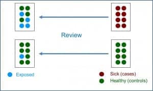
This approach would lead us to the design of a case-control study, which is an observational and analytical study in which sampling is done on the basis of presenting a certain disease or effect (the cases) and that group is compared with another group that it does not present it (the controls), in order to determine if there is a difference in the frequency of exposure to a certain risk factor between the two groups. These studies are of retrograde directionality and of mixed temporality, so they are retrospective. The most useful key to distinguish between them and cohort studies is the sampling of each one, based on the exposure in the cohort studies and based on the effect in the cases and controls.

In the attached figure you can see the typical design of a case-control study. These studies are based on a specific population from which a sample of cases that usually includes all diagnosed and available cases, are compared with a control group consisting of a balanced sample of healthy subjects from the same population. However, it is increasingly common to find variations in the basic design that combine characteristics of the cohort and case-control studies, comparing the cases that appear in a stable cohort over time with controls of a partial sample extracted from that same cohort.

Design’s variations

The best known of this type of mixed designs is that of nested in a cohort cases and controls. In these cases, we start with a well-known cohort in which we identify the cases that are occurring. Each time a case appears, it is paired with one or more controls also taken from the initial cohort. If we think about it briefly, it is possible that a subject that is initially selected as a control becomes a case over time (develop the disease under study). Although it may seem that this may bias the results, this should not be the case, since it is about measuring the effect of the exposure at the time of the analysis. This design can be done with smaller cohorts, so it can be simpler and cheaper. In addition, it is especially useful in very dynamic cohorts with many inputs and outputs over time, especially if the incidence of the disease under study is low.

Another variant of the basic design are the cohort and cases studies. In this type, we initially have a very large cohort from which we will select a smaller sub-cohort. The cases will be the patients that are produced in either of the two cohorts, while the controls will be the subjects of the smallest (and most manageable) sub-cohort. These studies have a method of analysis a little more complicated than the basic designs, since they have to compensate the fact that the cases are overrepresented because they come from the two cohorts. The great advantage of this design is that it allows studying several diseases at the same time, comparing the different cohorts of patients with the sub-cohort chosen as control.

Finally, one last variation that we are going to discuss is that of the polysemic case-cohort studies, also known as crossed cases and controls, also known as self-controlled cases. In this paired design, each individual serves as their own control, comparing the exposure during the period of time closest to the onset of the disease (case period) with the exposure during the previous period of time (control period). This study approach is useful when the exposure is short, with a foreseeable time of action and produces a disease of short duration in time. They are widely used, for example, to study the adverse effects of vaccines.

Association measure: odds ratio

As in cohort studies, case-control studies allow the calculation of a whole series of association and impact measures. Of course, here we have a fundamental difference with cohort studies. In cohort studies we started from a cohort without patients in which the patients appeared during the follow-up, which allowed us to calculate the risk of becoming ill over time (incidence). Thus, the quotient between incidents of exposed and not exposed gave us the risk ratio, the main measure of association.

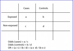
However, as can be deduced from the design of case-control studies, in these cases we cannot make a direct estimate of the incidence or prevalence of the disease, since the proportion of patients is determined by the selection criteria of the researcher and not by the incidence in the population (a fixed number of cases and controls are selected at the beginning, but we cannot calculate the risk of being a case in the population). Thus, before the impossibility of calculating the risk ratio, we will resort to the calculation of the odds ratio (OR), as you can see in the second figure.

The OR has a similar interpretation that the risk ratio, being able to value from zero to infinity. An OR = 1 means that there is no association between exposure and effect. An OR <1 means that exposure is a factor of protection against the effect. Finally, an OR> 1 indicates that the exposure is a risk factor, the higher the value of the OR.

Anyway and only for those who like getting into trouble, I will tell you that it is possible to calculate the incidence rates from the results of a case-control study. If the incidence of the disease under study is low (below 10%), OR and risk ratio can be comparable, so we can estimate the incidence in an approximate way. If the incidence of the disease is greater, the OR tends to overestimate the risk ratio, so we cannot consider them to be equivalent. In any case, in these cases, if we previously know the incidence of the disease in the population (obtained from other studies), we can calculate the incidence using the following formulas:

I0 = It / (OR x Pe) + P0

Ie = I0 x OR,

where It is the total incidence, Ie the incidence in exposed, I0 the incidence in not exposed, Pe the proportion of exposed, and P0 the proportion of not exposed.

Although the OR allows estimating the strength of the association between the exposure and the effect, it does not report on the potential effect that eliminating the exposure on the health of the population would have. For this, we will have to resort to the measures of attributable risk (as we did with cohort studies), which can be absolute or relative.

Impact measures

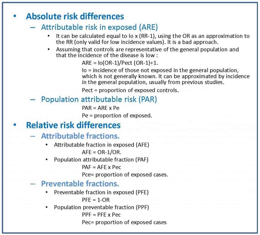
There are two absolute measures of attributable risk. The first is the attributable risk in exposed (ARE), which is the difference between the incidence in exposed and not exposed and represents the amount of incidence that can be attributed to the risk factor in the exposed. The second is the population attributable risk (PAR), which represents the amount of incidence that can be attributed to the risk factor in the general population.

On the other hand, there are also two relative measures of attributable risk (also known as proportions or attributable or etiological fractions). First, the attributable fraction in exposed (AFE), which represents the difference of risk relative to the incidence in the group of exposed to the factor. Second, the population attributable fraction (PAF), which represents the difference in risk relative to the incidence in the general population.

In the attached table I show you the formulas for the calculation of these parameters, which is somewhat more complex than in the case of cohort studies.

The problem with these impact measures is that they can sometimes be difficult for the clinician to interpret. For this reason, and inspired by the calculation of the number needed to treat (NNT) of clinical trials, a series of measures called impact numbers have been devised, which give us a more direct idea of the effect of the exposure factor on the disease. in study. These impact numbers are the number of impact in exposed (NIE), the number of impact in cases (NIC) and the number of impact in exposed cases (NIEC).

Let’s start with the simplest one. The NIE would be the equivalent of the NNT and would be calculated as the inverse of the absolute risk reduction or of the risk difference between exposed and not exposed. The NNT is the number of people who should be treated to prevent a case compared to the control group. The NIE represents the average number of people who have to be exposed to the risk factor so that a new case of illness occurs compared to the people who are not exposed. For example, a NIE of 10 means that out of every 10 exposed there will be a case of disease attributable to the risk factor studied.

The NIC is the inverse of the PAF, so it defines the average number of sick people among which a case is due to the risk factor. An NIC of 10 means that for every 10 patients in the population, one is attributable to the risk factor under study.

Finally, the NIEC is the inverse of the AFE. It is the average number of patients among which a case is attributable to the risk factor.

In summary, these three parameters measure the impact of exposure among all exposed (NIE), among all patients (NIC) and among all patients who have been exposed (NIEC). It will be useful for us to try to calculate them if the authors of the study do not do so, since they will give us an idea of the real impact of the exposure on the effect. In the second table I show you the formulas that you can use to obtain them.

As a culmination to the previous three, we could estimate the effect of the exposure on the entire population by calculating the number of impact on the population (NIP), for which we have only to do the inverse of the ARP. Thus, a NIP of 3000 means that for every 3,000 subjects of the population there will be a case of illness due to exposure.

Bias of case and control studies

In addition to assessing the measures of association and impact, when appraising a case-control study we will have to pay special attention to the presence of biases, since they are the observational studies that have the greatest risk of presenting them.

Case-control studies are relatively simple to make, have in general lower cost than other observational studies (including cohort studies), allow us to study various exposure factors at the same time and to know how they interact, and they are ideal for diseases of exposure factors with very low frequency. The problem with this type of design is that you have to be extremely careful selecting cases and controls, as it is very easy to commit a list of biases that, to this day, does not have a known end.

In general, the selection criteria should be the same for cases and controls, but as to be a case one has to be diagnosed and be available for the study, it’s very likely that cases are not fully representative of the population. For example, if the diagnostic criteria are not sensitive and specific enough we’ll get many false positives and negatives, with the consequent dilution of the effect of the exposure to the factor.

Other possible problem depends on the selection of incident (newly diagnosed) or prevalent cases. Prevalence based studies favor the selection of the survivors (as far as it’s known, no dead has agreed to participate in any study) and if survival is related to the exposure, the risk identified will be less than with incident cases. This effect is even more evident when the exposure factor is of good prognosis, a situation in which prevalence studies produces a greater overestimation of the association. As an example to better understand these issues, let’s suppose that the risk of suffer a stroke is higher the more one smokes. If we include only prevalent cases we’ll exclude the people dead of more severe heart attacks, which probably would be the one who smoke most, with which the effect of smoking could be underestimated.

But if selecting cases seems complicated, it’s nothing compared to a good selection of controls. Ideally, controls have had the same likely of exposure than cases or, put it another way, should be representative of the population from which the cases were extracted. In addition, this must be combined with the exclusion of those who have any illness related positively or negatively to the exposure factor. For example, If we want to waste our time and study the association between air passengers who have thrombophlebitis and prior aspirin ingestion, we must exclude from the study the controls that have any other disease being treated with aspirin, even if they had not taken it before the journey.

We have also to be careful with some habits of control selection. For instance, patients who go to the hospital for reasons different to that of study are at hand and tend to be very cooperative and, being sick, they surely better recall past exposure to risk factors. But the problem is that they are ill, so the pattern of exposure to risk factors can be different to the general population.

Another resource is to include neighbors, friend, relatives, etc. These usually are very comparable and cooperative, but we have the risk that there’re paired exposure habit that can alter study results. These entire problems are avoided taking controls from general population, but it is more costly in effort and money, they usually are less cooperative and, above all, much more forgetful (healthy people recall less about past exposures to risk factors), with so the quality of the information we obtain from cases and controls can be very different.

We’re leaving…

Just one more comment to end this theme so enjoyable. Case-control studies share a characteristic with the rest of the observational studies: they detect the association between exposure and effect, but they do not allow us to establish causality relations with certainty, for which we need other types of studies such as randomized clinical trials. But that is another story…