Fisher’s exact test.

Today we are going to remember one of the most beautiful stories, in my humble opinion, in the history of biostatistics. Although surely there are better stories, since my general historical ignorance is greater than the number of decimal places of the number pi.

A story of tea and numbers

Imagine we are at Rothamsted Station, an agricultural research center located in Harpenden, in the English county of Hertfordshire. We are at some moment in the beginning of the decade of the 20s of the last century.

Three scientists, very British themselves, are preparing to have tea. They are two men and one woman. This is Blanche Muriel Bristol, an expert on algae and mushrooms. With her is William Roach, a biochemist who is also married to Muriel.

The third one is a geneticist who has started working on the station and will eventually become famous for being one of the founders of population genetics and neo-Darwinism, as well as for a few other little things, like the concept of null hypothesis and hypothesis contrast. Yes, friends, he is the great Ronald Fisher.

Fisher prepares the teacups and gallantly offers the first to Muriel, who declines. She looks at Ronald and says: I like tea with milk, but only if you put milk in first. If done the other way around, it gives it a flavor that I don’t like at all.

Fisher thinks Muriel is teasing him, so he insists, but she’s still dug in her heels. I think then Fisher must have changed his mind and thought that Muriel was actually a bit of a fool, but the husband came to the rescue of his wife. William proposes to make 8 cups of tea and, at random, put the milk in first in 4 cups and then contrary in the rest.

To Fisher’s surprise, Muriel guesses the order in which the milk from the eight cups had been served, although she is not allowed to taste more than two cups at a time. Luck or a privileged palate?

This, which was one of the first randomized experiments in history, if not the first, left Fisher very thoughtful. So he developed a mathematical method to find out the probability that Muriel got it right by pure chance. And this method is the subject of our entry today: Fisher’s exact test.

Let’s clarify some concepts before

Before fully entering into Fisher’s exact test, we are going to clarify a series of concepts to understand well what we are going to do.

When we want to make a hypothesis contrast between two qualitative variables (in this case, to check their independence) we can use several tests that compare their frequencies or their proportions.

If we deal with independent data, we can choose an approximate test, such as the chi-square test, or an exact test, such as Fisher’s. If the deal with paired data, we can do a McNemar test (for 2×2 contingency tables) or use Cochran’s Q method (for 2xK tables).

And we have talked about exact and approximate tests. What does this mean?

The approximate tests calculate a statistic with a known probability distribution in order, according to its value, to know the probability that this statistic acquires values ​​equal to or more extreme than the observed one. It is an approximation that is made at the limit when the sample size tends to infinity.

For their part, exact tests calculate the probability of obtaining the observed results directly. This is done by generating all the possible scenarios that go in the same direction as the observed hypothesis and calculating the proportion in which the condition we are studying is fulfilled.

Which is better, an approximate test or an exact one?

Well, people who know about these things do not manage to agree.

The approximate methods are simpler from a computational point of view, but with the computational power of today’s computers, this argument does not seem to be a reason to choose them. On the other hand, the exact ones are more precise when the sample size is smaller or when some of the categories have a low number of observations.

But if the number of observations is very high, the result is similar using an exact method or an approximate one.

As a rule of thumb, it is recommended to use an exact test when the number of observations is less than 1000 or when there is a group with a number of expected events less than 5. However, if you have a computer, there is no reason to complicate your life: use an exact one.

All this does not mean that we cannot use an approximate test if the sample is small, but we will have to apply a continuity correction, as we saw in a previous post.

Fisher’s exact test

Fisher’s exact test is the exact method used when you want to study if there is an association between two qualitative variables, that is, if the proportions of one variable are different depending on the value of the other variable.

In principle, it seems that Fisher designed it with the idea of comparing two dichotomous qualitative variables. In simple terms, for use with 2×2 tables.

However, there are also extensions to the method to do it with larger tables. Many statistical programs are capable of doing this, although, logically, they put more stress on the computer. You can also find calculators available on the Internet.

Fisher’s exact test assumes the null hypothesis that the two variables are independent, that is, the values of one do not depend on the values of the other.

The only necessary condition is that the observations in the sample are independent of each other. This will be true if the sampling is random, if the sample size is less than 10% of the population size and if each observation contributes only to one of the levels of the qualitative variable.

Furthermore, the marginal frequencies of the rows and columns of the contingency tables of the different possible scenarios must remain fixed. Do not worry about this, it will be better understood when we see an example. If this is not true, we can continue to use the test, but it will no longer be exact and it will become more conservative.

Calculation of p-value

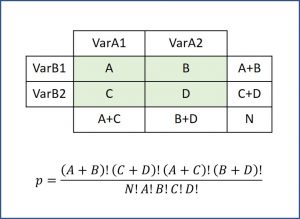
After much thought about the problem of tea and the skills of Muriel Bristol, the brilliant Fisher showed that he could calculate the probability of any of the contingency tables using the hypergeometric probability distribution, according to the formula in the figure.

Thus, Fisher’s exact test calculates the probabilities of all possible tables and adds those of the tables that have p values less than or equal to the observed one. This sum, multiplied by two, gives us the p-value for a two-tailed hypothesis contrast.

According to the value of p, we will only have to solve our hypothesis contrast in a similar way as we do with any other contrast test.

Let’s see an example

To finish understanding everything we have said, we are going to repeat the tea experiment but I, instead of Muriel, am going to ask my cousin to give us a hand; we have not caused him any troble for a long time.

Sure, I can’t make my cousin drink tea, so let’s see if he can tell the difference if what he’s drinking is Scottish or Irish whiskey. He claims that he is able to distinguish a Scottish from anything else.

So, to test his resistance to alcohol, as well as his palate skills, I randomly offer him 11 shots of Scottish and 11 shots of Irish.

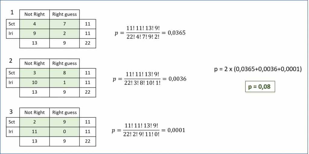
The results can be seen in the first table of the attached figure.

As you can see, it hits 7 of the 11 Scottish shots and only 2 of the 11 Irish ones. It seems that she is right in his statement and that he has a refined palate. But we, like Fisher did with Muriel, are going to see if he’s just been lucky.

As we have said above, it is necessary to calculate the possible tables that have a lower probability than the observed one and within the sense of our hypothesis. We will do this by reducing the minimum frequency of each of the columns until one of them reaches zero.

Also, we will adjust the other boxes so that the marginals remain constant. Otherwise, we already know that the test would no longer be exact. You can see the two possible tables until the hits with Irish whiskey reach zero.

Now we only have to calculate the probability of each table, add them all and multiply by two. We obtain a value of p = 0.08 for a bilateral contrast. As the null hypothesis says that the ability to hit is not influenced by the type of whiskey, we cannot deny that my cousin’s boast was just a matter of luck.

Do the calculation automatically

Coming to the end of this post, I¡d like to warn that no one ever thinks of doing a Fisher’s exact test manually. This absurd example is extremely simple, but surely our experiments are a bit more complex. Use a computer application or an Internet calculator.

Let’s solve the example using the R program.

First, we enter the data to build the contingency table with these two consecutive commands:

data <- data.frame(kindw = c(rep(“irh”,11), rep(“sct”,11)), hit = c(rep(TRUE,2), rep(FALSE,9), rep(TRUE,7), rep(FALSE,4)))

my_table <- table(data$kindw, data$hits, dnn = c(“Whisky”, “Hit”))

Finally, we perform Fisher’s exact test:

fisher.test(x = my_table, alternative = “two.sided”)

On the output screen, the program provides us with the p value (p = 0.08), its confidence interval and the odds ratio between the two variables. Remember that Fisher’s test only tells us if there is a statistically significant difference, but if we want to measure the strength of the association between the two variables we have to resort to other types of measures.

And if someone is looking for the value of the Fisher statistic among the program’s output data, I’m sorry to say that he or she has to re-read the entire post from the beginning.

As we have already said, exact tests calculate probability directly without the need for prior calculation of a statistic that follows a known probability distribution. The Fisher’s statistic does not exist.

We’re leaving…

And here we are going to leave it for today. We have seen how Fisher’s exact test allows us to study the independence of two qualitative variables but requires one condition: that the marginal frequencies of rows and columns remain constant.

And this can be a problem, because in many biological experiments we will not be able or not sure of meeting this requirement. What happens then? As always, there are several alternatives.

The first, keep using the test. The drawback is that it is no longer an exact test and loses its advantages over approximate tests. But we could use it.

The second is to use another contrast test that does not lose power when the marginals of the table are not fixed, such as Barnard’s test. But that is another story…