Geometric mean

We already know that the arithmetic mean is the most famous of the measures of central tendency of a distribution, so it should come as no surprise that it is involved in so many statistical and mathematical procedures.

However, the mean has a small flaw: it is easily bias by the presence of extreme values in the data distribution. To put it a little more technically, it is not very robust in the presence of outliers.

For these cases, it may be more convenient to use other measures of central tendency that are more robust. Today we are going to talk about one of them, the geometric mean. And, to do so, we are going to assume that we have become microbiologists.

A little experiment

Let us imagine that we are in our laboratory looking for a way to enrich a culture medium to more easily detect the presence of Fildulastrum fildulastrii, the causal germ of that terrible disease that is fildulastrosis.

We are going to seed a series of plates with the bugs and, to compare the plates with the different enrichment media, we are going to calculate the mean of the bugs that grow in each series.

For example, we have five plates that we have enriched with a certain medium and we count the colonies that we obtain in each one: 1,000, 100, 100,000, 100 and 1,000.

Now I ask you: what is the average growth with this culture medium?

The least thoughtful of you will rush to calculate the arithmetic mean, which is 20,440 colonies per dish.

And so I would ask you: do you really think that 20,440 is a good measure of central tendency for this distribution of values? If you think about it, you will see that it is not. The problem is that we have an extreme value, 100,000, and the arithmetic mean is irresistibly drawn towards it.

To calculate a more accurate measure of central tendency we need something more robust against the presence of outliers. Specifically, we need to resort to the geometric mean.

Geometric mean

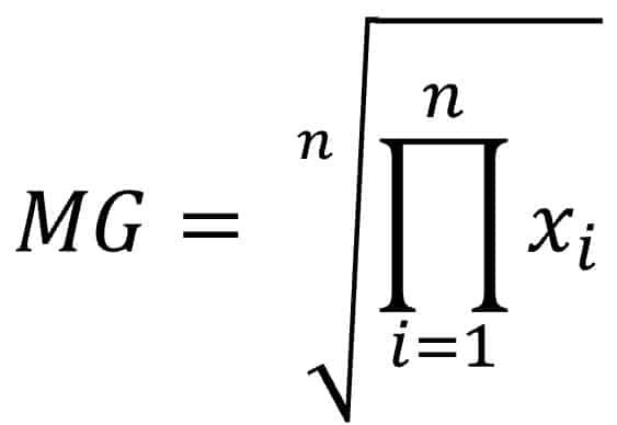
The geometric mean of a series of n numbers is the nth root of the roblema of all the numbers.

For those who know how to appreciate the beauty of mathematical language, what has been said above can be expressed with the following formula:

The geometric mean is often used when the values ​​of the distribution change multiplicatively, and not additively. This makes it ideal for averaging geometric progression data, such as ratios, compound interest in economics, and, as in our case, bacterial growths in microbiology.

For example, if a company has grown 15%, 22%, 14%, 18% and 12% in the last 5 years, the correct thing to do would be to calculate the geometric mean to give a measure of average growth for the 5 years. We can use the R program to calculate it:

(15*22*14*18*12)^0.2 = 15.84.

The average growth is 15.84%. I clarify, just in case, that raising to 0.2 (1/5) is the same as doing the fifth root.

Now let’s apply it to our roblema:

(1000*100*100000*100*1000)^0.2 = 1,000.

It is now clear, 1000 seems to us a more accurate measure of central tendency for this distribution.

An unexpected relationship

To finish this post, we are going to see one of those unexpected relationships that the magic of mathematics offers to us from time to time. And it turns out that the geometric mean is closely related to logarithms. Let’s see it.

Although it may seem strange, Napier invented logarithms in the 17th century to facilitate mathematical calculations. The simplest way, in my humble opinion, to say what a logarithm is, is to say that the logarithm of a number indicates the exponent to which a number (the base) must be raised to obtain the original number.

Let’s look at an example to understand it better. The base 10 logarithm of 100 is equal to 2:

log10(100) = 2

This is so because 2 is the number to which the base (10) must be raised to to obtain the original number (100).

It turns out that the product of n numbers is equal to the sum of their logarithms, so the logarithm of the geometric mean will be equal to the arithmetic mean of the sum of logarithms.

In this way, to calculate the geometric mean, we can:

1. Add the logarithms of the numbers in the distribution.

2. Divide them by the total numbers (n) to calculate the arithmetic mean.

3. Calculate the antilogarithm or, what is the same, the exponential function to obtain the geometric mean.

Let’s see how we would solve our example with this other method, using the R program:

geometric.mean <- exp(mean(log(c(1000, 100, 100000, 100, 1000))))

The result would be what we already know, 1,000.

We’re leaving…

And here we will leave it for today.

We have seen some of the uses of the geometric mean, which should not be confused with another very similar robust measure of central tendency, the harmonic mean. The harmonic mean is more used in situations in which it is necessary to average paths of equal length with different times, as well as to average multiples or quotients.

In addition, there are other robust measures of central tendency that we have not discussed at all, such as trimmed mean, winsorized, weighted, etc. But that is another story…