Assessment of diagnostic tests.

We describe how to assess the power of diagnostic tests: sensitivity, specificity, predictive values, and likelihood ratios.
A brother-in-law of mine is very concerned with a dilemma he’s gotten into. The thing is that he’s going to start a small business and he wants to hire a security guard to stay at the entrance door and watch for those who take something without paying for it. And the problem is that there’re two candidates and he doesn’t know what of both to choose.
One of them stops nearly everyone, so no burglar escapes. Of course, many honest people are offended when they are asked to open their bags before leaving and so next time they will buy elsewhere. The other guard is the opposite: he stops almost anyone but the one he spots certainly brings something stolen. He offends few honest people, but too many grabbers escape. Difficult decision…
Why my brother-in-law comes to me with this story?. Because he knows that I daily face with similar dilemmas every time I have to choose a diagnostic test. And the thing is that there’re still people who think that if you get a positive result with a diagnostic tool you have a certain diagnostic of illness and, conversely, that if you are sick to know the diagnostic you only have to do a test. And things are not, nor much less, so simple. Nor is gold all that glitters neither all gold have the same quality.
Assessment of diagnostic tests
Let’s see it with an example. 
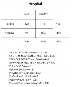
Now suppose I perform a study with my hospital patients with a new diagnostic test for a particular disease and I get the results showed in the table below (the sick are those with a positive reference test and the healthy those with a negative one).
Sensibility and specificity
Let’s start with the easy part. We have 1598 subjects, 520 out of them sick and 1078 healthy. The test gives us 446 positive results, 428 true (TP) and 18 false (FP). It also gives us 1152 negatives, 1060 true (TN) and 92 false (FN). The first we can determine is the ability of the test to distinguish between healthy and sick, which leads me to introduce the first two concepts: sensitivity (Se) and specificity (Sp).
Se is the likelihood that the test correctly classifies a patient or, in other words, the probability that a patient gets a positive result. It’s calculated dividing TP by the number of sick. In our case it equals 0.82 (if you prefer to use percentages you have to multiply by 100). Moreover, Sp is the likelihood that the test correctly classifies a healthy or, put another way, the probability that a healthy gets a negative result. It’s calculated dividing TN by the number of healthy. In our example, it equals 0.98.
Someone may think that we have assessed the value of the new test, but we have just begun to do it. And this is because with Se and Sp we somehow measure the ability of the test to discriminate between healthy and sick, but what we really need to know is the probability that an individual with a positive results being sick and, although it may seem to be similar concepts, they are actually quite different.
Predictive values
The probability of a positive of being sick is known as the positive predictive value (PPV) and is calculated dividing the number of patients with a positive test by the total number of positives. In our case it is 0.96. This means that a positive has a 96% chance of being sick.
Moreover, the probability of a negative of being healthy is expressed by the negative predictive value (NPV), with is the quotient of healthy with a negative test by the total number of negatives. In our example it equals 0.92 (an individual with a negative result has 92% chance of being healthy).
And from now on is when neurons begin to be overheated. It turns out that Se and Sp are two intrinsic characteristics of the diagnostic test. Their results will be the same whenever we use the test in similar conditions, regardless of the subjects of the test.
But this is not so with the predictive values, which vary depending on the prevalence of the disease in the population in which we test. This means that the probability of a positive of being sick depends on how common or rare the disease in the population is. Yes, you read this right: the same positive test expresses different risk of being sick, and for unbelievers, I’ll put another example.
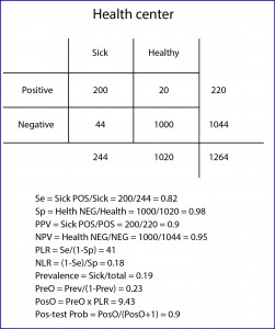
Suppose that this same study is repeated by one of my colleagues who works at a community health center, where population is proportionally healthier than at my hospital (logical, they have not suffered the hospital yet). If you check the results in the table and bring you the trouble to calculate it, you may come up with a Se of 0.82 and a Sp of 0.98, the same that I came up with in my practice. However, if you calculate the predictive values, you will see that the PPV equals 0.9 and the NPV 0.95.
And this is so because the prevalence of the disease (sick divided by total) is different in the two populations: 0.32 at my practice vs 0.19 at the health center. That is, in cases of highest prevalence a positive value is more valuable to confirm the diagnosis of disease, but a negative is less reliable to rule it out. And conversely, if the disease is very rare a negative result will reasonably rule out disease but a positive will be less reliable at the time to confirm it.
We see that, as almost always happen in medicine, we are moving on the shaking ground of probability, since all (absolutely all) diagnostic tests are imperfect and make mistakes when classifying healthy and sick. So when is a diagnostic test worth of using it?.
If you think about it, any particular subject has a probability of being sick even before performing the test (the prevalence of disease in his population) and we’re only interested in using diagnostic tests that increase this likelihood enough to justify the initiation of the appropriate treatment (otherwise we would have to do another test to reach the threshold level of probability to justify treatment).
Likelihood ratios
And here is when this issue begins to be a little unfriendly. The positive likelihood ratio (PLR), also known as positive probability ratio, indicates how much more probable is to get a positive with a sick than with a healthy subject. The proportion of positive in sick patients is represented by Se.
The proportion of positives in healthy are the FP, which would be those healthy without a negative result or, what is the same, 1-Sp. Thus, PLR = Se / (1 – Sp). In our case (hospital) it equals 41 (the same value no matter we use percentages for Se and Sp). This can be interpreted as it is 41 times more likely to get a positive with a sick than with a healthy.
It’s also possible to calculate NLR (negative), which expresses how much likely is to find a negative in a sick than in a healthy. Negative patients are those who don’t test positive (1-Se) and negative healthy are the same as the TN (the test’s Sp). So, NLR = (1 – Se) / Sp. In our example 0.18.
A ratio of 1 indicates that the result of the test doesn’t change the probability of being sick. If it’s greater than 1 the probability is increased and, if less than 1, decreased.
This is the parameter used to determine the diagnostic power of the test. Values > 10 (or < 0.01) indicates that it’s a very powerful test that supports (or contradict) the diagnosis; values from 5-10 (or 0.1-0.2) indicates low power of the test to support (or disprove) the diagnosis; 2-5 (or 0.2-05) indicates that the contribution of the test is questionable; and, finally, 1-2 (0.5-1) indicates that the test has not diagnostic value.
Post-test probability
The likelihood ratio doesn’t express a direct chance, but it allows us to calculate the odds of being sick before and after testing positive for the diagnostic test. We can calculate the pre-test odds (PreO) as the prevalence divided by its complementary (how much probably is to be sick than not to be).
In our case it equals 0.47. Moreover, the post-test odd (PosO) is calculated as the product of the prevalence by the PreO. In our case, it is 19.27. And finally, following the reverse mechanism that we use to get the PreO from the prevalence, post-test probability (PosP) would be equal to PosO / (PosO +1). In our example it equals 0.95, which means that if our test is positive the probability of being sick changes from 0.32 (the prevalence) to 0.95 (post-test probability).
If there’s still anyone reading at this point, I’ll say that we don’t need all this gibberish to get post-test probability. There are multiple websites with online calculators for all these parameters from the initial 2 by 2 table with a minimum effort. I addition, the post-test probability can be easily calculated using a Fagan’s nomogram. What we need to know is how to properly assess the information provided by a diagnostic tool to see if it’s useful because of its power, costs, patient discomfort, etc.
We’re leaving…
Just one last question. We’ve been talking all the time about positive and negative diagnostic tests, but when the result of the test is quantitative, we must set what value we consider positive and what negative, with which all the parameters we’ve seen will vary depending on these values, especially Se and Sp. And to which of the parameters of the diagnostic test must we give priority?. Well, that depends on the characteristics of the test and on the use that we pretend to give to it, but that’s another story…
