Step by Step. Probability calculations with a normal distribution.

We already know that the normal distribution is one of the most used in biomedicine, since a large number of random variables follow this distribution. Although the density function of this probability distribution is rather unsympathetic, it is make up by the fact that the distribution can be characterized with only two parameters, its mean and its variance, with which we can perform multiple probability calculations.
We are going to carry out some examples of these calculations, using the R program and with the help of its R-Commander graphical interface. Although R has the advantages of being very powerful and totally free, its exclusive use from the command line can be a bit harsh for the uninitiated.
Some preliminars
Of course, to perform calculations on a data set, the first thing we are going to need is that data set.
In real life we would already have them. It would be the results of our study that we would import from R to do the statistical study.
On this occasion, we are going to make the data by generating a random distribution with R.
It must be said, first of all, that statistical programs do not generate random numbers, but pseudo-random numbers, performing calculations from a previous number that is usually referred to as the seed.

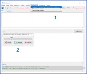
First we launch R. Second, we launch R-Commander with the library(Rcmdr) command. Third, we select the menu option Distributions -> Set the seed of the random number generator. In the pop-up window that appears we select, for example, 24814. You can see it in the first figure. This can also be done with the command set.seed(24814).

We already have it all. Let’s get started!
Step 1. Check the normality of the data
We already have our database, called “pas”, which we are going to assume is a record of the systolic blood pressure of 1000 adolescents.
We are not going to go into how to do the basic descriptive statistical study here. We will only do a minimal numerical summary to verify that data are correct. We open the menu Statistics-> Summaries-> Numerical Summaries.
We see that our variable have a mean of 119.78 (we stay with 120) and a standard deviation of 11.83 (we stay with 12). The program also provides us with the median, the quartiles, the interquartile range, and the sample size.
We are going to check that they follow a normal distribution. We open the menu Statistics-> Summaries-> Normality test… In the pop-up window we mark, for example, the Shapiro-Wilk test. When we accept, the program gives us a statistic W = 0.99 with a value of p = 0.58.
Since p> 0.05, we cannot reject the null hypothesis which, for this test, assumes that data are normally distributed. But we already know that these numerical tests are not very powerful, so it is convenient to complement this result with some graphic method.
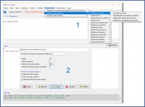
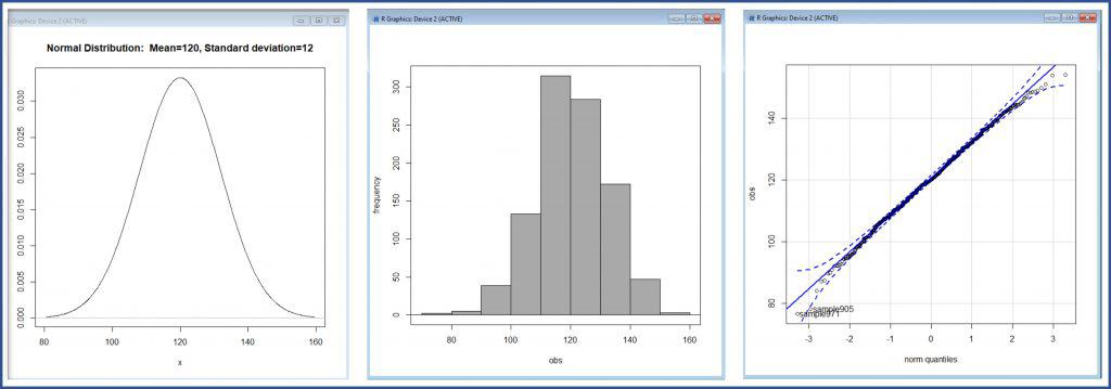
We select Distributions-> Continuous distributions-> Normal distribution-> Graph of the normal distribution…, Graphs-> Histogram, and Graphs-> Graph of comparison of quantiles… We thus obtain the graphical representation of the distribution, its histogram and the graph of theoretical quantiles, respectively, which you can see in the third figure.
Both the graphical representation of the curve and the shape of the histogram are compatible with a normal distribution. Furthermore, in the third graph, the points follow the diagonal quite well, which means that the quantiles of the distribution resemble quite well the theoretical ones if the distribution were normal.
In summary, we can assume that our data follow a normal distribution.
Step 2. Direct information that the normal distribution provides
Knowing that the arterial pressure of our adolescents follows a normal distribution of mean m=120 and standard deviation s=12, we can already draw a series of conclusions.
In a normal distribution, the values are centered symmetrically around the mean. 68% out of the population is grouped around m ± 1 s, 95% out of the population between m ± 2 s, and 99% between m ± 3 s, approximately.
With minimal calculations, we know that 68% out of our adolescents will have a pressure between 108 and 132 mmHg, 95% between 96 and 144 mmHg and 99% between 84 and 156 mmHg. In addition, only 2.5% out of the population will have a pressure less than 96 mmHg, and another 2.5%, greater than 144 mmHg.
Finally, we could estimate the value in the population from which the sample were extracted by calculating its confidence interval.
The 95% confidence interval of a mean is calculated according to the following formula:
95 CI = m ± 1.96 se
“se” represents the standard error of the mean, which is calculated, in turn, by dividing the standard deviation by the square root of the sample size.
Thus, we can already do the calculation:
95 CI = 120 ± 1.96 x (12 / square root of 1000)
If we solve the above equation, we obtain that, with 95% confidence, the mean value of systolic blood pressure of the population’s adolescents will be between 119.25 and 120.74 mmHg.
For the most puristic, we assume that we know the population’s variance and that it is equal to that of our sample. Otherwise, we would have had to use the quasi-standard deviation or, better still, use a Student’s t distribution to calculate the interval (although with such a large sample we would get essentially the same result).
Step 3. Probability calculation
Let’s imagine that we are interested in knowing the percentage of the population who have a pressure included in a certain interval. For example, between 90 and 135 mmHg. In other words, what is the probability that a randomly selected individual will have a systolic blood pressure between 90 and 135 mmHg.
We are going to calculate it with R through the menu Distributions-> Continuous distributions-> Normal distribution-> Cumulative normal probabilities…:
– Less than 90 mmHg: we mark 90 in the box “value (s) of the variable”, 120 in “mean” and 12 in “standard deviation”. What tail do we select? Since we want the probability of values less than 90, we select the left tail. R tells us that the probability is 0.0062.
– Greater than 135 mmHg: we mark 135 in the box “value (s) of the variable”, 120 in “mean” and 12 in “standard deviation”. What tail do we select? Since we want the probability of values greater than 135, this time we select the right tail. R tells us that the probability is 0.1056.
Since the total probability is 1 (100%), we know that P(<90) + P(90-135) + P(> 135) = 1. If we solve the equation, we obtain that P(90-135) = 0.8882. Rounding up, 89% out of our adolescents have a systolic blood pressure between 90 and 135 mmHg.
In other words, if we draw an individual at random, there is a 0.89 (89%) probability that their blood pressure is in the range of 90 to 135 mmHg.
Step 4. To standardize simplifies the calculations
The standard normal distribution is one that has a mean of 0 and a variance of 1, and which is usually represented as N (0,1).
Its great advantage is that it makes calculations much easier. In our example, a priori we do not know how many young people will have a blood pressure greater than 144 mmHg. However, in a standard distribution we know, without having to calculate, that the probability of having more than 2 (which is the same as more than 2 standard deviations) is 0.025 (2.5%).
Given the above, it is easy to understand that it will be simpler to calculate the probabilities of the standardized values. To do this, the mean of the distribution is subtracted from each value and the result is divided by the standard deviation. We thus calculate what we usually call the z-score, which represents the number of standard deviations that each value separates from the mean of the distribution.
Thus, for 90, z-score = -2.5; for 135, z-score = 1.25. We already know from a glance that it will be very unlikely to find someone with a pressure less than -2.5 and that there will not be much beyond a 10% above 1.25. Thus, the proportion of those within the range of -2.5 to 1.25 will be around 90%.
Of course, this is not done for rounding. We can use the same method as before to calculate the exact value of the probability. Do it and you will see how the same thing comes out.
The advantage, in addition to being more intuitive when the characteristics of the normal distribution are known, is that, in the case of not having a computer at hand, with a single probability table we can do the calculations for any normal distribution we desire. We just have to standardize it.
We’re leaving…
We have seen how to check that our data set follows a normal distribution and thus be able to calculate the probability of finding certain values.
But what if our data are not normally distributed? Well, we would have several options, from trying to transform them to using other probability distributions. But that is another story…

