Step by Step. Chi-square test for independence.
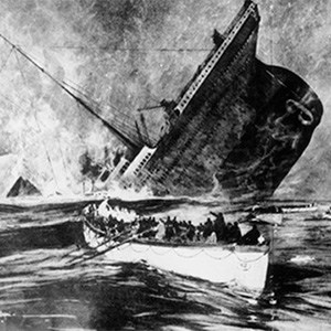
Who doesn’t know the story of the Titanic, the unsinkable ship that finally sinked into the icy waters of the North Atlantic?
When it was built, the RMS Titanic was the largest passenger ship of the time. In addition to all the luxuries and comforts of its, it had the most advanced security measures of its time, such as the hull bulkheads and the watertight gates, which should ensure the impossibility that the ship could sink.
However, after setting sail from Southampton on April 10, 1912, on April 14 at 11:40 p.m. it collided with an iceberg 600 kilometers south of Newfoundland, sinking 3 hours later and killing 1,496 of the 2208 people. who were traveling on board.
The history of the Titanic teaches us, among many other things, how bad overconfidence is. Nobody could imagine that a ship of the time could sink like that. It was probably that overconfidence that caused the dangers of the trip to be misjudged until it was too late.
But it also teaches us how enormously the assessment of an event can vary depending on the point of view from which it is made. What, for the passengers and for all humanity, was an immense tragedy, for the lobsters in the Titanic’s fish tank all was a true miracle.
A classy shipwreck
One of the reasons for the high death toll in the Titanic wreck was caused by the fact that the ship did not have lifeboats for even half of the passengers. Although the boats were the most innovative of the time, the quantity was determined, incomprehensibly, by the weight of the ship and not by the number of travelers.
In addition, there has always been some controversy about whether the poor and the rich suffered the same fate in the face of misfortune. Although, as the saying goes, they were all in the same boat, and that there are things that money cannot buy, when you look at the numbers of survivors you cannot help but feel uneasy.
Of course, the percentage of deaths in the three classes is not exactly the same, but could the observed differences be due to chance or did the class really influence the probability of survival?
We are going to try to answer this question using the R program, with its R-Commander interface and a data set called TitanicSurvival.
Some preliminary preparations
As you already know, R works based on packages, which are a kind of libraries with certain functionalities.
Many of these packages include datasets, which can be used to test statistical techniques of your choice. We are going to use the TitanicSurvival dataset, from the carData package. This data set includes information on 1309 passengers, collecting in four fields whether they survived or not, their sex, age and the class in which they were traveling.
First, we launch R. Second, we launch R-Commander with the library(Rcmdr) command.
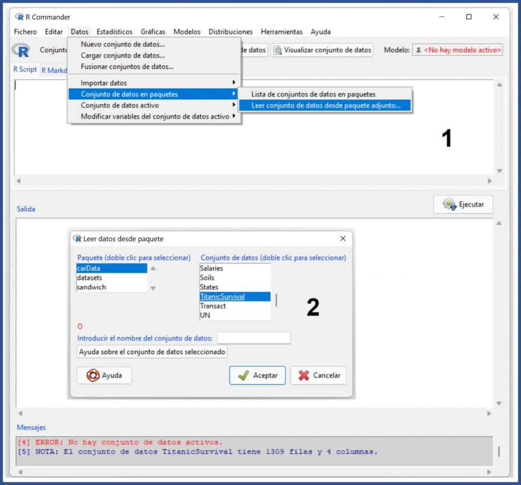
In the first figure I show you how to load the data once the R-Commander interface is open. We go to the menu Data->Load data in packages->Read dataset from attached package… In the pop-up window, select carData as package and TitanicSurvival as dataset. Click OK and you will have the data in the active data set.
If you do not know which package the set or data belongs to or if you want to know what datasets are loaded in R, you can see the complete list by selecting the menu option Data-> Load data in packages->List of data sets in packages.
Step 1. Descriptive analysis of data
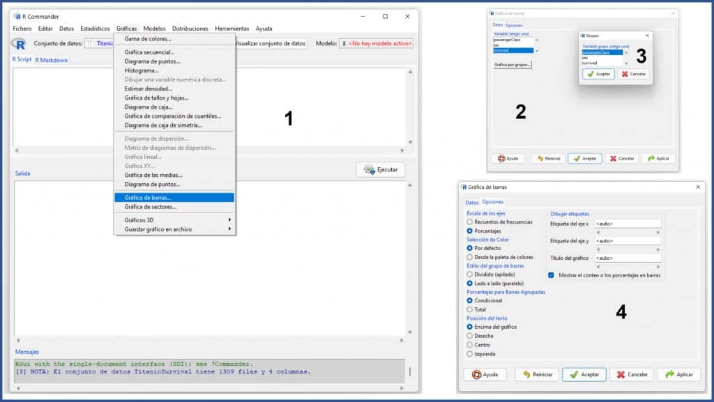
First, we are going to graphically represent the two variables. Since these are two nominal variables, we will make a bar diagram. We select the menu option Graphs->Bar graph… (next figure). In the pop-up window we mark the variable “survived” and click on the button "Graph by groups" to select “passengerClass”.
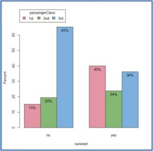
Once this is done, we open the “Options” tab and mark the options “Axes scale” by percentages and “Bar group style” side by side. We press accept and we obtain the diagram in the next figure.
At first glance, it seems that the distribution of classes is not the same between those who survive and those who do not. We will now proceed to carry out our hypothesis testing to check if these differences are statistically significant or can be explained by pure chance.
We already saw in a previous post that the choice of the statistical test depends on the type of variables to be compared, on whether we are dealing with independent samples or with paired data and, in some cases, on the probability distribution that data follows.
In this case we want to compare two qualitative variables: survival (survived), with two categories (yes and no), and class (passengerClass), with three categories (first, second, and third).
In addition, we want to know if these two variables are independent of each other or if they are related, so that the value of one of them influences the value of the other. To do this, the two simplest choices are the chi-square test for independence of two variables and Fisher’s exact test.
Today we are going to perform a chi-square test and save Fisher’s exact test for another time.
Step 2. Chi-square test of independence
In the first place, we are going to do it in the simplest way, letting R build for us the contingency table with the two variables under study. We can only do this in this way if we have the data set we want to study loaded.
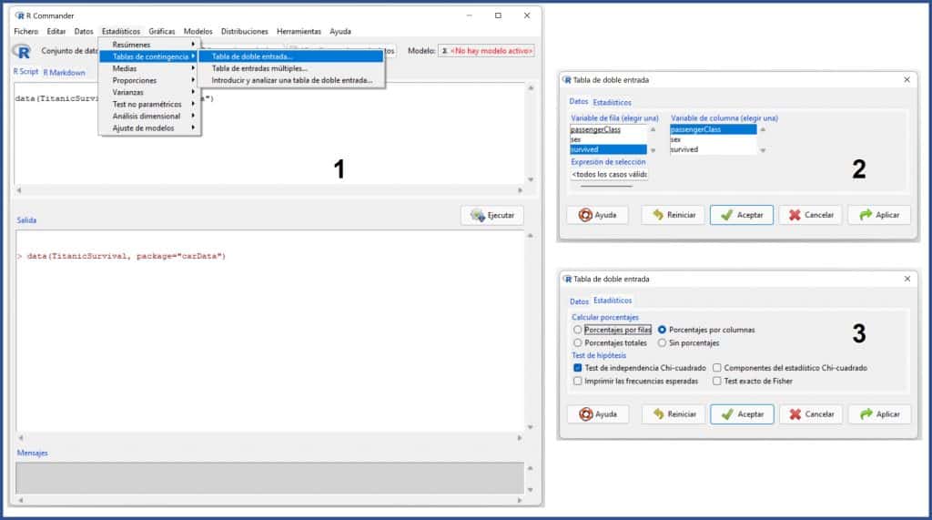
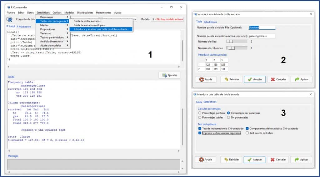
We open the menu Statistics->Contingency tables->Double entry table… In the pop-up window we select the row variable (survived) and the column variable (passengerClass). Then we click on the Statistics tab and mark the option "percentage by columns". We do this so that it tells us, in addition to the total numbers, the percentage of survival in each class. Thus we can study the results of the two variables.
As shown in the previous figure, at the bottom of this window there are several more options, which are related with the test. We are only going to mark the option "Chi-square independence test" and press accept.
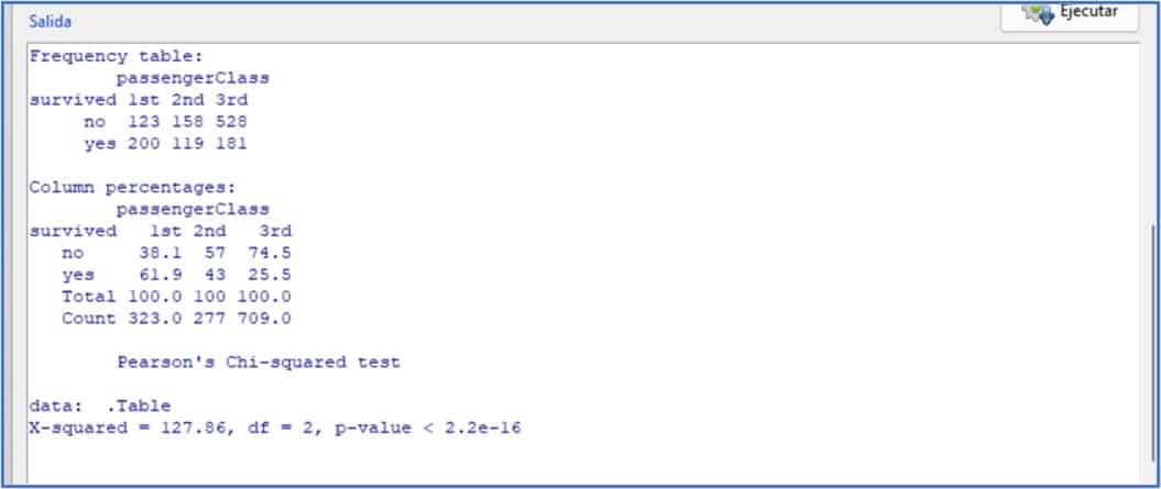
In the attached figure you can see the results shown in R’s output window.
First, we have the table of absolute frequencies. We can see that 200 out of the 323 first class survive, 119 out of the 277 second class and 181 out of the 709 third class. Although it already seems that there are differences, we will see this better in the second table, which shows us the percentages by columns.
We can see that 61.9% out of first-class passengers survive, 43% out of second-class passengers and 25.5% out of third-class passengers. Now we can see the differences clearly, with an increase in the probability of surviving in the upper classes, but could this difference be due to chance?
To answer this question we look at the last line of the results. It tells us that the value of the chi-square statistic is 127.86, with 2 degrees of freedom. If the class did not influence survival, this value should be close to 1. The probability (the value of p) of finding this value or a higher one due to chance is 2.2×10⁻¹⁶, that is, practically 0 (and surely less than 0.05).
The null hypothesis of the chi-square test assumes that the two variables are independent. As the p is less than 0.05, we can reject the null hypothesis and reach an important conclusion: as long as the data are representative of reality, if the Titanic is ever refloated and we want to travel in it, better let it be first class. Just in case.
Step 3. Manual introduction of contingency table
Imagine that we do not have the database, but we know the results, either in absolute frequencies or in percentages. In this case, R will not build for us the contingency table, but it does allow us to do it manually.
We select the menu option Statistics->Contingency tables->Enter and analyze a double-entry variable… (see next figure). In the pop-up window, we enter the names of the variables, mark the number of rows and columns, and fill in the table that is offered to us at the bottom of the window.
Next, we click on the Statistics tab and mark the options that interest us. We are going to select the option "Percentages by columns" and mark all the options in the "Hypothesis test" section except the Fisher exact test which, as we have already said, we are going to leave for another time.
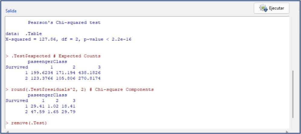
In the last figure you can see the results output. In this case, we have asked R to also show us the expected theoretical values if the null hypothesis of independence were true. We can see how they deviate from the real values that we have obtained.
As with the previous calculation, chi-square has a value of 127.86, with 2 degrees of freedom, which means a value of p close to 0. There are no surprises, we get the same result doing it both ways.
We’re leaving…
We have seen in this post how to test the independence of two qualitative variables using the chi-square test.
We saw in a previous post that the chi-square test makes an approximation using a known probability distribution, which is none other than the chi-square distribution. On the other hand, we can use one of the exact tests, which calculate the probability directly, generating all the possible scenarios in which the condition we want to study occurs.
The exact test to perform this hypothesis test is the so-called Fisher’s exact test, which, although it has higher computational requirements, should be the first-choice contrast test, especially with small samples. But that is another story…

