Cochran’s Q.

Polysemy is one of the characteristics of language, you know, that party of meanings in which a word decides to wear multiple disguises. Take, for example, the letter Q.

Q is the seventeenth letter of the Latin alphabet, commonly used in languages such as Spanish, English, French and many others. You all know it, it is similar to the letter O, but with an added tail that gives it a distinctive touch.

Anyway, when I think of Q, my mind quickly drifts to the world of movies and spy novels and I remember Q, the technological genius behind the extravagant adventures of James Bond. Q is the mastermind behind MI6’s most ingenious gadgets. But let’s be fair, Q is not only the toy supplier for Agent 007, but also the character who adds a touch of wit and cunning to Bond’s elegant and dangerous life.

You see that Q is much more than a simple letter of the alphabet. But today we are not going to talk about semantics, much less about films. Because Q is not just a letter or a surname, it is also the key to unravelling the statistical mysteries that haunt our meta-analyses. Like a quantum detective, another Q, Cochran’s Q, helps us reveal the truth hidden in the data, or at least, it tries to do so amidst so much uncertainty and statistical heterogeneity.

But don’t worry, we won’t need a magnifying glass or a raincoat to follow this exciting path. Make yourself comfortable and prepare to walk through a world where numbers make their movements and hypotheses are unravelled. Let’s go there.

A prior clarification

Before starting to talk about how to measure heterogeneity in a meta-analysis, I think it is worth making a prior clarification, because here we once again encounter the polysemy of language, and the term “heterogeneity” can have two meanings.

First, there may be differences between the primary studies of a meta-analysis in terms of population, intervention, comparison and outcome (the classic components of the structured clinical question, PICO). This heterogeneity, which we can call clinical, can be reduced when we design our study by asking an appropriate research question, but there is no point in trying to correct it in the results analysis phase.

Apples should not be mixed with pears. If we find ourselves in this situation, the correct thing to do is to limit ourselves to doing a qualitative synthesis of our systematic review and refrain from doing a quantitative synthesis or meta-analysis.

Secondly, we may find ourselves faced with what we call statistical heterogeneity, due to the precision of the estimates made in the meta-analysis. This heterogeneity, which can be high even if the studies are very homogeneous from a clinical point of view, must always be considered when analysing the results.

Statistical heterogeneity is responsible for the variability between studies in the meta-analysis. Because, once again, we can also find more than one source of variability.

Sources of variability in meta-analysis

When considering the sources of variation between the effects observed in the primary studies of a meta-analysis, we can use two different models: the fixed effect model and the random effects model.

The fixed effect model assumes that the effect we want to estimate is the same in the populations from which the samples with which the primary studies are carried out come. In this way, the differences observed between the effects of the studies are due solely to chance.

For its part, the random effects model assumes that each population has its specific effect, so that these random effects are considered random variables that follow a certain distribution, and their inclusion in the model helps to improve the precision of the estimates and to consider variability between studies.

Thus, there are two sources of variability under the random effects model. On the one hand, our inseparable companion, chance. On the other hand, the variability between studies. And here Cochran’s Q comes into play, helping us to differentiate between random or sampling error from that due to real differences between the different meta-analysis studies.

Cochran’s Q

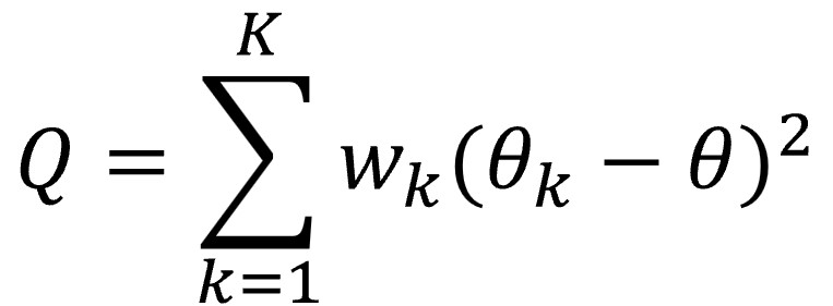
Back in the 1950s, Cochran defined his famous Q by resorting to a very beloved tool in the world of statistics, which is none other than the sum of the squares of the differences between the observed value and the calculated one, the residuals. In this case, the sum of the squares of the differences between the effect of each study and the summary effect measure calculated according to the fixed effect model is calculated, weighting each difference by the contribution of each study to the summary effect result.

Since a picture is worth a thousand words (or so they say), I show you the formula below.

Let’s look a little more at the formula, although many would like to forget it as soon as possible. The letter θ represents the summary effect measure calculated by applying, as we have already said, a fixed effect model, while θ_k represents the effect of each primary study. K represents the number of studies, with k being each individual study. Finally, w_k is the weight of each study, calculated as the inverse of its variance (what is usual in the fixed effect model).

We can easily understand that the value of Q will increase as the number of studies increases. Furthermore, when weighted by the inverse of the variance (the standard error of the effect), studies with a very small error will greatly influence Q value, even if the effect value differs little from the summary measure.

The obtained Q value can be used to measure the excess variation that we can attribute exclusively to chance or, in other words, the heterogeneity between studies. But what value of Q will indicate that there is heterogeneity beyond that explained by sampling error?

The answer is that there is no value that we can establish in a general way, but it will depend on each case, so, to better understand how to calculate it, we are going to do a small simulation with completely invented data.

Experimenting with Cochran’s Q

Let’s see how the value of Q behaves under the assumptions of absence and presence of heterogeneity. To do this, we are going to use the R program to calculate the distribution that the Q values follow in these two situations. I will be writing the R commands, in case someone wants to replicate the experiment at the same time we are doing it.

Absence of heterogeneity

Let’s start by assuming that there is no heterogeneity. This implies that the value of the residuals (the difference between the effect of each study and the summary measure with the fixed effect model) is distributed normally around the value of the summary measure, with a mean of 0 and a certain variance, which, in this case, we are going to assume that it is 1. Thus, we can say that the residuals are distributed according to a standard normal, N(0,1).

Assuming our meta-analysis has 35 studies, we could calculate the residual values with R’s rnorm() function:

residuals <- rnorm(n = 35, mean = 0, sd = 1)

This would give us the values of the residuals for our meta-analysis, but what we are interested in is knowing how these residuals behave if we repeat the study many times, in order to calculate the sampling distribution of the residuals and, from it, that of Q’s sampling distribution. We can simulate repeating the meta-analysis 10,000 times with the following command:

fixed_err <- replicate(10000, rnorm(n = 35, mean = 0, sd = 1))

Finally, remembering the formula for Q, we can calculate its value in each of these 10,000 meta-analyses. For simplicity, let’s assume that the weight of all studies is equal to 1:

Q_fixed <- replicate(10000, sum(rnorm(n = 35, mean = 0, sd = 1) ^ 2))

Let no one worry too much if they do not fully understand how we do the simulation. The interesting thing comes now.

Since it is a weighted sum of squares, Q can only acquire positive values, and we know that it follows, approximately, a chi-square distribution with a number of degrees of freedom equal to the number of studies minus one (K – 1). I take this opportunity to remember that the chi-square distribution is characterized by having a mean equal to the number of degrees of freedom and a variance equal to twice the degrees of freedom.

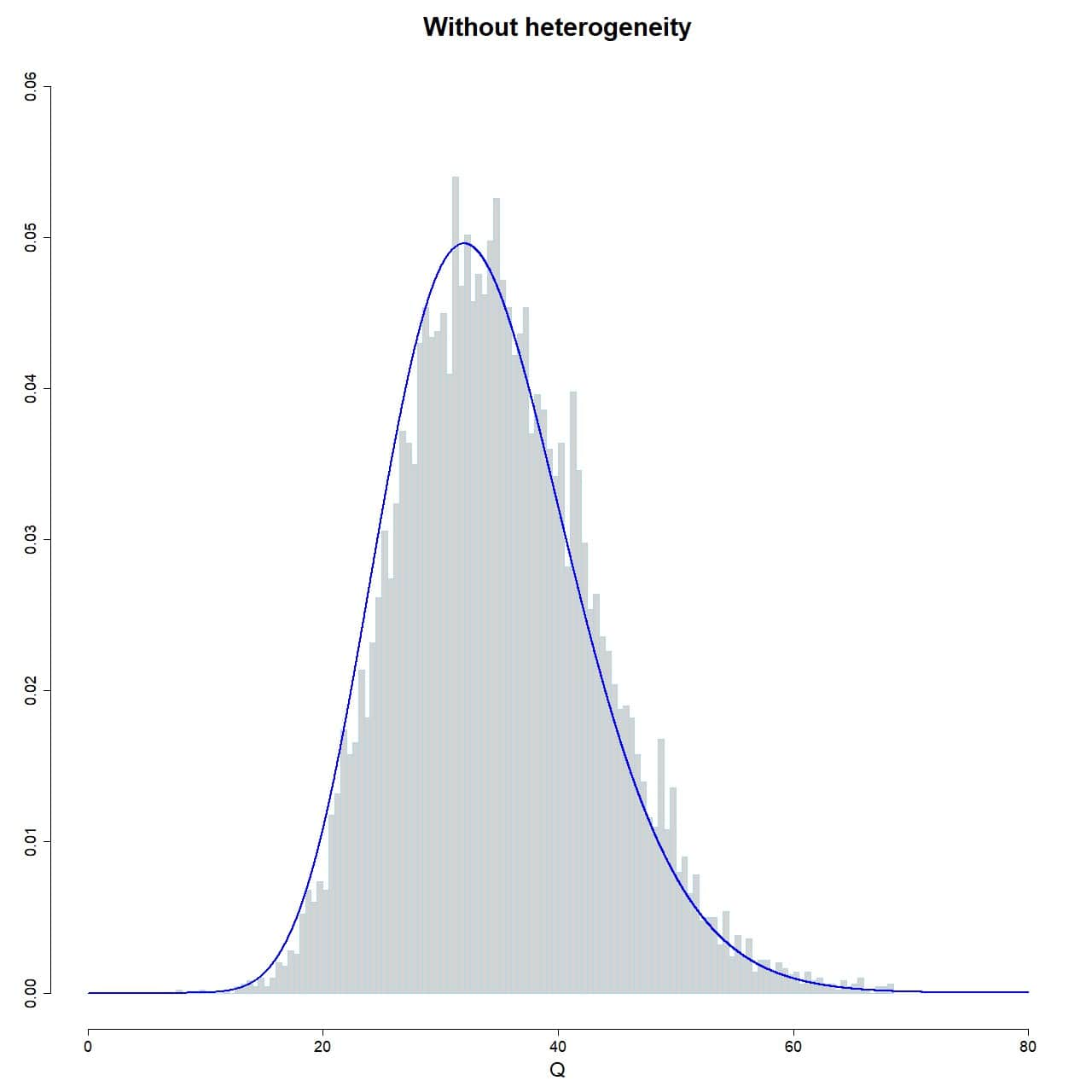
To check that our simulation works, we plot the histogram of the sampling distribution of Q, superimposing the curve of the chi-square distribution with 35-1 degrees of freedom:

hist(Q_fixed, xlab="Q", prob = TRUE, breaks = 100, ylim = c(0, 0.06), xlim = c(0, 80), ylab = "", main = "Without heterogeneity", border="lightblue")

lines(seq(0, 80, 0.01), dchisq(seq(0, 80, 0.01), df = 35-1), col = "blue", lwd = 2)

As you can see in attached figure, the Q values of the 10,000 simulated studies reasonably follows the distribution, so there are no surprises so far.

Presence of heterogeneity

In this case, we must assume that the residuals have two components of variability: chance and variability between studies. We can calculate it in a similar way as we did before, but adding a second component:

residuals <- rnorm(n = 35, mean = 0, sd = 1) + rnorm(n = 35, mean = 0, sd = 1)

We now calculate the Q values for the 10,000 simulated meta-analyses under the assumption that heterogeneity exists:

Q_random <- replicate(10000, sum((rnorm(n = 35, mean = 0, sd = 1) +

rnorm(n = 35, mean = 0, sd = 1))^2))

Now we only have to do the graphical representation, in a similar way to what we did before:

hist(Q_random, xlab="Q", prob = TRUE, breaks = 100, ylim = c(0, 0.06), xlim = c(0, 160), ylab = "",  main = "With heterogeneity", border = "pink")

lines(seq(0, 100, 0.01), dchisq(seq(0, 100, 0.01), df = 35-1), col = "red", lwd = 2)

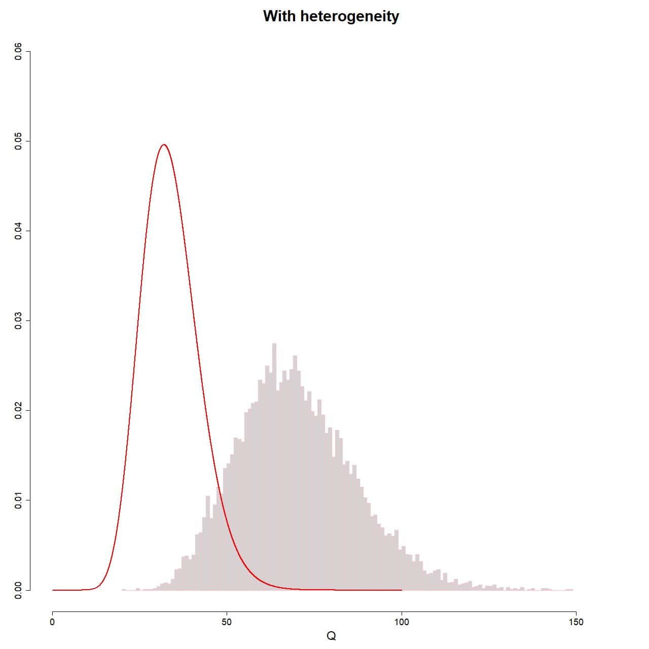
The result is shown in attached figure. As you can see, this time the sampling distribution of the Q values does not fit the theoretical chi-square distribution. To do this, the assumption of non-heterogeneity should be met, which, as we know, is not met on this occasion.

Well, it is this deviation from the theoretical distribution when there is variability between studies what we can leverage to determine if there is heterogeneity between primary studies.

The hypothesis test for Cochran’s Q

We are going to carry out a hypothesis test under the assumption that the null hypothesis of absence of heterogeneity is met.

What we do is calculate the value of Cochran’s Q with the effects of the studies in our meta-analysis. Ideally, under the null hypothesis assumption, the expected value is K-1 (the mean of the distribution), although we already know that the value will almost always be different, if only due to random error.

We will only have to calculate the probability of finding a value of Q as extreme or more extreme than the one we have found, just by chance. If this probability (the p-value) is greater than 0.05, we will not be able to reject the null hypothesis and we will assume that there is no heterogeneity.

On the contrary, if p < 0.05, we will reject the hypothesis and conclude that there is statistical heterogeneity between the primary studies in the meta-analysis.

Let’s look at an example. Suppose that in our meta-analysis of 35 studies we have calculated the value of Cochran’s Q, which is equal to 52.5. To obtain the value of p, we can execute the following command in R:

pchisq(q = 52.5, df = 34, lower.tail = FALSE)

This command gives us the probability of obtaining, just by chance, a value of Q like the one we have obtained or greater (the area under the curve of the right tail). The program gave us a p-value = 0.02. We can reject the null hypothesis and conclude that there is heterogeneity between the primary studies.

As always, the important thing is to understand the concept. The statistics program with which we carry out the meta-analysis will be in charge of all these calculations.

Variations on a theme by Cochran

Cochran’s Q is a widely used measure to detect heterogeneity and, roughly, we can say that the greater the variability between studies, it will be greater.

The problem is that its value is not very intuitive to assess the intensity of this variability, which is why two more estimators have been developed, which aim to be easier to interpret. These are I² and H², which can be calculated from the value of Q.

The I² statistic

I² defines the percentage of variability in the size of the effects that is not caused by random error or, in other words, that is due to heterogeneity. It is calculated according to the following formula.

We already know that, if there is no heterogeneity, the expected value of Q is K-1 (the mean of the chi-square distribution). If we subtract K-1 (the expected value due to random error) from the value of Q (observed) and divide it by the total Q, it will give us what proportion of the value of Q that is not explained by chance.

In the event that Q is less than the expected mean (K-1), we assume that I², which is usually multiplied by 100 and expressed as a percentage, is equal to 0 (it is logical, the proportion of variability due to heterogeneity may be more or less high, but never less than 0%).

The value of I² can range from 0 to 100%, with the limits of 25%, 50% and 75% usually being considered to delimit when there is low, moderate and high heterogeneity, respectively.

An advantage of the I² is that it does not depend on the units of measurement of the effects or the number of studies, so, unlike what happens with Cochran’s Q, it does allow comparisons with different effect measures and between different meta-analyses with different number of studies.

If we calculate the value of I² in our example with 35 studies and a Q value of 52.5, we see that it is 35.2%, indicating moderate heterogeneity.

The H² statistic

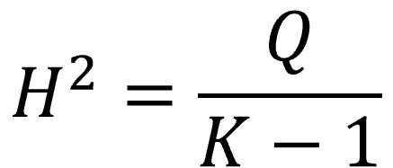
This statistic, much less famous than the previous one, is also calculated from the value of Q and represents the ratio between the observed value (Q) and the one expected under the assumption of the null hypothesis (K-1, the mean of the distribution):

In this case it is not necessary to make any correction when the value of Q is less than K-1. When there is no heterogeneity, H² ≤ 1. Values greater than 1 indicate variability between studies.

In our example, with a Q value of 52.5 and 35 studies, H² is equal to 1.54, which indicates the existence of heterogeneity.

We’re leaving…

And this is where we have come today.

We have seen how the Cochran’s Q value is usually used to detect heterogeneity between studies in a meta-analysis, although it has some defects, such as depending on the number and precision of the studies.

I², for its part, is somewhat less sensitive to these effects and easier to interpret, but still depends on the precision of the studies included in the meta-analysis. If the studies have very large samples, the random error will tend to 0, but Q will increase when weighted by the inverse of the variance and the value of I² will tend towards 100%.

That is why it is not a good idea to limit ourselves to calculating the values of Q and I² (or H², which behaves similarly to I²), so many authors advise completing the assessment of heterogeneity with the calculation of τ² (which is not , strictly speaking, a measure of heterogeneity) and prediction intervals. But that is another story…