Comparison of proportions.

We review the methods for comparison of proportions: chi-square, Fisher’s exact test and approximation to a normal.

This expression has its origin in the crazy habit that came to Romans for making roads connecting the capital of the Empire with the outlying provinces. There was a time any road took you to Rome, hence the saying.

Today the roads can take you anywhere, but the phrase is preserve for using it when we mean that there are several ways to achieve the same end. For example, if we want to know if there is dependence between two variables and if the difference between them is statistically significant. There are always several ways to get our precious p.

A pill of history

And to prove it, we’ll start with an absurd and impossible example, for which I’ll have to use my time machine. So, as it’s all about Rome, we go to the year 216 BC, in full Second Punic War, and plan a study to know who were smarter, the Romans or the Carthaginians.

To do it, we select a sample of 251 Romans and 249 Carthaginians we catch absent-minded at the Battle of Cannae and had them an IQ test to see how many have an intelligence quotient greater than 120, which we’ll consider to be pretty smart.

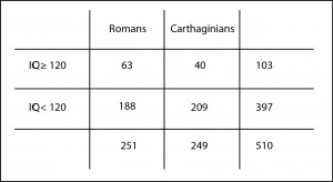
You can see the results in the table I attached. We can see that 25% of the Romans (63 out of 251) and 16% of the Carthaginians (40 out of 249) may be classified as smart. At first glance one would think than Romans were smarter but, of course, there is always the possibility that this difference is due to random sampling error.

So we set our null hypothesis that all of them are equally intelligent, we choose an statistic whose probability distribution under the null is known, we calculate its value, and we compute the value of p. If p is lower than 0.05 we’ll reject the null hypothesis and will conclude that Romans were smarter. By the way, if it’s greater than 0.05 we cannot reject the null, so we have to conclude that both of them were equally intelligent and that the observed difference is due to chance.

Comparison of proportions

The first statistic that comes to mind is the chi-squared test. As we know, it assesses the differences among expected and observed values and gives us a value that follows a known distribution (the chi-squared), so we can calculate its p-value. In this way, we build the contingency table with expected and observed values and we come up with a chi-squared equals to 6.35.

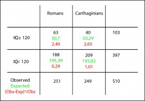
Now we can calculate the p-value using, for instance, one of the probability calculators available on the Internet, obtaining a p-value = 0.01. As it’s lower than 0.05 we reject the null hypothesis and conclude that Romans were indeed smarter than Carthaginians, which would explain why they won the three Punic Wars, although the second one remained in their craw for a long time.

Another way to do the same thing

But we have said that all roads lead to Rome. And another way to reach the p-value would be to compare the two proportions and to check if their difference is statistically significant. Again, our null hypothesis is that there’s no difference between the two, so the difference, if the null is true, should be zero.

Thus, what we have to do is calculate the difference between the proportions and standardize the results dividing it by its standard error, thus getting a z-value that will follows a normal probability distribution.

The formula is

With it we obtain a z-value = 2.51. If we use another probability calculator to compute the probability outside de mean ± z (the contrast is bilateral), will get a p-value pf 0.01. Indeed, the same p-value that we obtained with the chi-squared test.

But this should not surprise us. At the end of the day, the p-value is just the probability of being wrong rejecting the null hypothesis (type I error). And as the null hypothesis is the same no matter we use chi-squared test or z comparison, the probability of type I error should be the same in both cases.

But, in addition, there is another curiosity. The value of the chi-squared (6.35) is exactly the squared of the value we obtained for z (2.51). But this should not surprise us either knowing that chi-squared and normal distributions are related. If we squared all the values of a normal distribution of frequencies and we plot the results, we’ll get a chi-squared frequency distribution. Funny, isn’t it?

We could also perform a Fisher exact test rather than a chi-squared test and would get similar results.

We’re leaving…

And with this we’ll leave Romans and Carthaginians alone. Jus to say that there’re still more ways to assess whether the difference in proportions is significant or not. We could have calculated the confidence interval of the difference or the interval of their quotient (relative risk) or even the interval of their odds ratio, and check if the intervals include the null value to determine if they were statistically significant. But that’s another story…