Conditionals transposition fallacy.

Conditionals transposition fallacy arises from a poor understanding of the concept of p-value and conditional probability.
A fallacy is an argument that appears valid but is not. Sometimes it’s used to deceive people and to give them a pig in a poke, but most of the time it is used for a much sadder reason: ignorance.
Today we will talk about one of these fallacies, very little known, but wherein we fall with great frequency when interpreting results of hypothesis testing.
Increasingly we see that scientific journals provide us with the exact value of p, so we tend to think that the lower the value of p the greater the plausibility of the observed effect.
To understand what we are going to explain, let us first remember the logic of falsification of the null hypothesis (H0). We start from a H0 that the effect does not exist, so we calculate the probability of finding such extreme results than those we found just by chance, given that H0 is true.
This probability is the p-value, so that the smaller, the less likely that the result is due to chance and therefore most likely that the effect is real. The problem is that however small the p, there is always a probability of making a type I error and reject H0 being true (or what is the same, get a false positive and take for good an effect than does not really exist).
It is important to note that the p-value only indicates whether we have reached the threshold for statistical significance, which is a totally arbitrary value. If we get a threshold value of p = 0.05 we tend to think of the following four possibilities:
- That there is a 5% chance that the result is a false positive (that H0 is true).
- That there is a 95% chance that the effect is real (that H0 is false).
- The probability that the observed effect is due to chance is 5%.
- The rate of type I error is 5%.
However, all of this is wrong and we are falling in the inverse fallacy or the conditionals’ transposition fallacy. Everything is a problem of misunderstanding the conditional probabilities. Let’s see it slowly.
Conditionals tranposition fallacy
We are interested to know what the probability of H0 being true is given the results we have obtained. Expressed mathematically, we want to know P (H0 | results). However, the p-value is what gives us the probability of obtaining our results given that the null hypothesis is true, that is, P (result | H0).
Let’s see a simple example. The probability of being Spanish if you’re Andalusian is high (it should be 100%). The inverse is lower. The likelihood of having a headache if you have meningitis is high. The inverse is lower. If events are frequent, the probability will be higher than if they are rare. So, as we want to know P (H0 | results), we assess the baseline probability of H0 to avoid overestimating the evidence supporting that the effect is true.
If we think about it, it’s pretty intuitive. The probability of H0 before the study is a measure of a subjective belief that reflects their plausibility based on previous studies. Let’s think that we want to test an effect that we believe very unlikely to be true. We’ll assess with caution a p-value less than 0.05, albeit significant. On the contrary, if we are convinced that the effect exists, with little p we will be satisfied.
In short, to calculate the probability that the effect is real we will have to calibrate the p value with the value of the baseline probability of H0, which will be assigned by the investigator or by previous available data. Needless to say that there is a mathematical method to calculate the posterior probability of H0 according to their baseline probability and the p-value, but it would be rude to put a huge formula at this point of post.
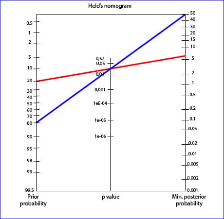
 Instead, we will use a simpler method, using a graphic resource named Held’s nomogram that you can see in the figure.
To use the Held’s nomogram all we have to do is to draw a line from the previous probability that we think has H0 and prolong it through the p-value until reach the value of the posterior probability.
Imagine one study with a marginal value of p = 0.03 in which we believe the probability of H0 is 20% (we believe there is an 80% chance that the effect is real). If we draw the line we’ll get a minimum probability of H0 of 6%: there is a 94% chance that the effect is real.
On the other hand, think of another study with the same value of p but in which we think the probability of the effect is lower, for example, 20% (the probability of H0 is 80%). For the same value p, the subsequent minimum probability of H0 is 50%, and then there is a 50% chance that the effect is real. We see how the posterior probability changes with the previous probability.
We’re leaving…
And here we leave it. Surely this Held’s nomogram has reminded you of another much more famous nomogram but with a similar philosophy: the Fagan’s nomogram. This is used to calculate the post-test probability based on the pretest probability and the likelihood ratio of a diagnostic test. But that is another story…
