Hypothesis contrast.

The steps of hypothesis contrast are reviewed: null and alternative hypotheses, choice of statistic, calculation of the p-value and decision.
Every day we face many situations where we always act in the same way. For us, it’s always the same old story. And this is good, because these situations allow us to take an action routinely, without having to think about it.
The problem with these same-old-story situations is that we have to understand very well how to do them. Otherwise, we can do and get anything but what we want.
Hypothesis contrast
Hypothesis contrast is an example of one of these situations. It’s always the same: the same old story. And yet, at first it seems more complicated than it really is. Because, regardless of the contrast we’re doing, the steps are always the same: to establish our null hypothesis, to choose the appropriate statistic for each situation, to use the corresponding probability distribution to calculate the probability of that value of the statistic chosen and, according to that probability value, deciding in favor of the null hypothesis or the alternative. We will discuss these steps one by one using an example in order to better understand all these stuff.

The null hypothesis
First, we set our null and alternative hypotheses. As we know, when doing a hypothesis testing we can reject the null hypothesis if the statistic chosen has a certain probability. What we cannot do is ever accept it, only to reject it. This is why we usually set the null hypothesis as the opposite of what we want to show, to be able to reject what we don’t want to show and so accept what we want to show.
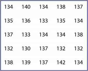
In our example we’re going to set the null hypothesis that our students’ stature is equal to the town’s average and that the difference found is due to sampling error, to pure chance. Moreover, the alternative hypothesis says that there is an actual difference and that our children are shorter.
Choosing the statistical test
Once established the null and alternative hypothesis we have to choose the appropriate statistic for this hypothesis testing. This case is one of the simplest, the comparison of two means, ours and the population’s mean. In this case, our standardized mean respect of the population’s mean follows a Student’s t distribution, according to the following expression:
t = (group mean – population mean) / standard error of the mean
So, we substitute the mean value for our value (135.4 cm), the population’s mean for 138 and the standard error for its value (the standard deviation divided by the squared root of the sample size) and we obtain a value of t = -4.55.
p-value
Now we have to calculate the probability that t has a value of -4.55. If we think about it, we’ll see that in the case that the two mean were equal t has a value of zero. The more different they are, the far from zero the t-value will be. We need to know if that deviation from zero to -4.55 could be due to chance. To do this, we calculate the probability that the value of t = -4.55, using a table of the Student’s distribution or a computer program, getting a value of p = 0.0001.
Contrast
We already have the p-value, so we only have to do the last step, to see if we can reject the null hypothesis. The p-value indicates the probability that the observed difference between the two means is due to chance. As it’s lower than 0.05 (lower than 5%), we feel confident enough to say that it’s not due to chance (or at least that it’s very unlikely), so we reject the null hypothesis that the difference is due to chance and embrace the alternative hypothesis that the two means are really different. Conclusion: ours are the tiny schoolchildren in town.
And this is all about the hypothesis testing of equality of two means. In this case, we have done a t-test for one sample, but the punch line if the dynamics of hypothesis testing. It’s always the same: the same old story. What change from time to time, logically, is the statistic and probability distribution we use for every occasion.
We’re leaving…
To conclude, I just want to draw your attention to another method we could have used to calculate if the means were different. This is just to use our beloved confidence intervals. We could have calculated the confidence interval of our mean and check if it included the population’s mean, in which case we would have concluded that they were similar. If the population’s mean would have been out of the range of the interval, we would have rejected the null hypothesis, reaching logically our same conclusion. But that’s another story…
