The least squared method.

The other day I was trying to measure the distance between Madrid and New York in Google Earth and I found something unexpected: when I tried to draw a straight line between the two cities, it twisted and formed an arc, and there was no way to avoid it.

I wondered if what Euclid said about the straight line being the shortest path between two points would not be true. Of course, right away, I realized where the error was: Euclid was thinking about the distance between two points located in a plane and I was drawing the minimum distance between two points located in a sphere. Obviously, in this case the shortest distance is not marked by a straight line, but an arc, as Google showed me.

And since one thing leads to another, this led me to think about what would happen if instead of two points there were many more. This has to do, as some of you already imagine, with the regression line that is calculated to fit a point cloud. Here, as it is easy to understand, the line cannot pass through all the points without losing its straightness, so the statisticians devised a way to calculate the line that is closest to all points on average. The method they use the most is the one they call the least squared method, whose name suggests something strange and esoteric. However, the reasoning for calculating it is much simpler and, therefore, no less ingenious. Let’s see it.

The least squared method

The linear regression model makes it possible, once a linear relation has been established, to make predictions about the value of a variable Y knowing the values of a set of variables X₁, X₂, … X_n. We call the variable Y as dependent, although it is also known as objective, endogenous, criterion or explained variable. For their part, the X variables are the independent variables, also known as predictors, explanatory, exogenous or regressors.

When there are several independent variables, we are faced with a multiple linear regression model, while when there is only one, we will talk about simple linear regression. To make it easier, we will focus, of course, on the simple regression, although the reasoning also applies to multiple one.

As we have already said, linear regression requires that the relationship between the two variables is linear, so it can be represented by the following equation of a straight line:

Here we find two new friends accompanying our dependent and independent variables: they are the coefficients of the regression model. β₀ represents the model constant (also called the intercept) and is the point where the line intersects the ordinate axis (the Y axis, to understand each other better). It would represent the theoretical value of variable Y when variable X values zero.

For its part, β₁ represents the slope (inclination) of the regression line. This coefficient tells us the increment of units of variable Y that occurs for each increment of one unit of variable X.

We meet chance again

This would be the general theoretical line of the model. The problem is that the distribution of values is never going to fit perfectly to any line, so when we are going to calculate a determined value of Y (y_i) from a value of X (x_i) there will be a difference between the real value of y_i and the one that we obtain with the formula of the line. We have already met with random, our inseparable companion, so we will have no choice but to include it in the equation:

Although it seems a similar formula to the previous one, it has undergone a profound transformation. We now have two well-differentiated components, a deterministic and a stochastic (error) component. The deterministic component is marked by the first two elements of the equation, while the stochastic is marked by the error in the estimation. The two components are characterized by their random variable, x_i and ε_i, respectively, while x_i would be a specific and known value of the variable X.

Let’s focus a little on the value of ε_i. We have already said that it represents the difference between the real value of y_i in our point cloud and that which would be provided by the equation of the line (the estimated value, represented as ŷ_i). We can represent it mathematically in the following way:

This value is known as the residual and its value depends on chance, although if the model is not well specified, other factors may also systematically influence it, but that does not change what we are dealing with.

Let’s summarize

Let’s recap what we have so far:

1. A point cloud on which we want to draw the line that best fits the cloud.
2. An infinite number of possible lines, from which we want to select a specific one.
3. A general model with two components: one deterministic and the other stochastic. This second will depend, if the model is correct, on chance.

We already have the values of the variables X and Y in our point cloud for which we want to calculate the line. What will vary in the equation of the line that we select will be the coefficients of the model, β₀ and β₁. And what coefficients interest us? Logically, those with which the random component of the equation (the error) is as small as possible. In other words, we want the equation with a value of the sum of residuals as low as possible.

Starting from the previous equation of each residual, we can represent the sum of residuals as follows, where n is the number of pairs of values of X and Y that we have:

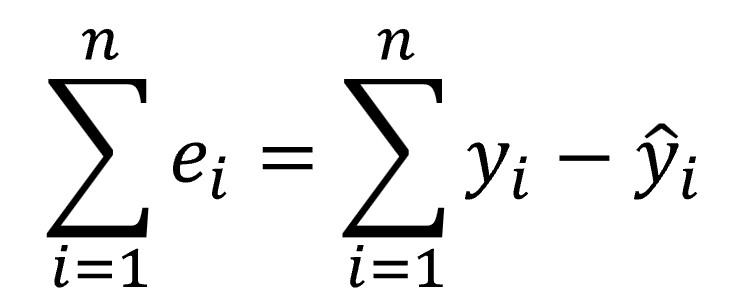
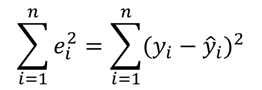
But this formula does not work for us. If the difference between the estimated value and the real value is random, sometimes it will be positive and sometimes negative. Furthermore, its average will be zero or close to zero. For this reason, as on other occasions in which it is interesting to measure the magnitude of the deviation, we have to resort to a method that prevents from negatives differences canceling out with the positives ones, so we calculate these squared differences, according to the following formula:

We already got it!

At last! We already know where the least squares method comes from: we look for the regression line that gives us the smallest possible value of the sum of the squares of the residuals. To calculate the coefficients of the regression line we will only have to expand the previous equation a little, substituting the estimated value of Y for the terms of the regression line equation:

and find the values of b₀ and b₁ that minimize the function. From here the task is a piece of cake, we just have to set the partial derivatives of the previous equation to zero (take it easy, let’s save the hard-mathematical jargon) to get the value of b₁:

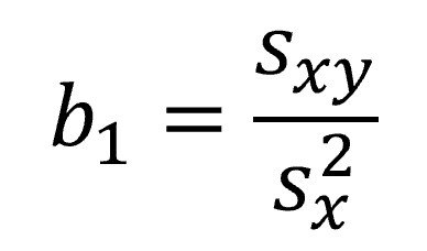
Where we have in the numerator the covariance of the two variables and, in the denominator, the variance of the independent variable. From here, the calculation of b₀ is a breeze:

We can now build our line that, if you look closely, goes through the mean values of X and Y.

A practical exercise

And with this we end the arduous part of this post. Everything we have said is to understand what the least squares mean and where the matter comes from, but it is not necessary to do all this to calculate the linear regression line. Statistical packages do it in the blink of an eye.

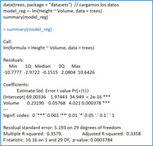
For example, in R it is calculated using the function lm(), which stands for linear model. Let’s see an example using the “trees” database (girth, volume and height of 31 observations on trees), calculating the regression line to estimate the volume of the trees knowing their height:

modelo_reg <- lm(Height~Volume, data = trees)

summary(modelo_reg)

The lm() function returns the model to the variable that we have indicated (reg_model, in this case), which we can exploit later, for example, with the summary() function. This will provide us with a series of data, as you can see in the attached figure.

First, the quartiles and the median of the residuals. For the model to be correct, it is important that the median is close to zero and that the absolute values of the residuals are distributed evenly among the quartiles (similar between maximum and minimum and between first and third quartiles).

Next, the point estimate of the coefficients is shown below along with their standard error, which will allow us to calculate their confidence intervals. This is accompanied by the values of the t statistic with its statistical significance. We have not said it, but the coefficients follow a Student’s t distribution with n-2 degrees of freedom, which allows us to know if they are statistically significant.

Finally, the standard deviation of the residuals is provided, the square of the multiple correlation coefficient or determination coefficient (the precision with which the line represents the functional relationship between the two variables; its square root in simple regression is the Pearson’s correlation coefficient), its adjusted value (which will be more reliable when we calculate regression models with small samples) and the F contrast to validate the model (the variance ratios follow a Snedecor’s F distribution).

Thus, our regression equation would be as follows:

Height = 69 + 0.23xVolume

We could already calculate how tall a tree could be given a specific volume that was not in our sample (although it should be within the range of data used to calculate the regression line, since it is risky to make predictions outside this range).

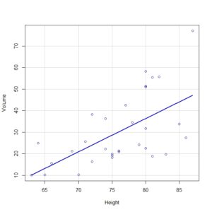
Also, with the scatterplot(Volume ~ Height, regLine = TRUE, smooth = FALSE, boxplots = FALSE, data = trees) command, we could draw the point cloud and the regression line, as you can see in the second figure.

And we could calculate many more parameters related to the regression model calculated by R, but we will leave it here for today.

We’re leaving…

Before finishing, just to tell you that the least squares method is not the only one that allows us to calculate the regression line that best fits our point cloud. There is also another method that is that of the maximum likelihood, which gives more importance to the choice of the coefficients that with more compatibility with the observed values. But that is another story…