Resampling techniques: bootstrapping.

Bootstrapping is a resampling technique that allows calculations that are impossible in another way when the sample is small.

That is bootstrapping. It’s an idea impossible to perform, in addition to a swearword, of course.

The name is related to the straps that boots have on their top, especially those cowboy’s boots we see in the movies. Bootstrapping is a term that apparently refers to the action of elevated oneself from the ground by simultaneously pulling the straps of both boots. As I said, it’s an impossible task because of the Newton’s third law, the famous action-reaction law.

Bootstrapping

Bootstrapping is a resampling technique that is used in statistics with increasing frequency thanks to the power of today’s computers, which allow calculations that could previously be inconceivable. Perhaps his name has to do with its character of impossible task because bootstrapping is used to make possible some tasks that might seem impossible when the size of our sample is very small or when the distributions are highly skewed, as obtaining confidence intervals or perform statistical significance tests or any other statistics in which we are interested.

As you recall from when we calculate the mean’s confidence interval, in theory we can do the experiment of obtaining multiple samples from a population to calculate the mean of each sample and represent the distribution of those means obtained from multiple samples. This is called the sampling distribution, whose mean is the estimator of the parameter in the population and whose standard deviation is called the standard error of the statistic that, in turn, will allow us to calculate the confidence interval we want. Thus, extraction of repeated samples from the population allows us to make descriptions and statistical inferences.

Well, bootstrapping is similar, but with one key difference: the successive samples are taken from our sample and not from the population from which it comes. The procedure follows a series of repetitive steps.

First, we draw a sample from the original sample. This sample must be collected using sampling with replacement, so some items may not be selected and others may be selected more than once in each sampling. It is logical, if we have a sample of 10 elements and extract 10 items without replacement, the sample obtained is equal to the original, so that we won’t get anything new.

From this new sample we get the desired statistic and use it as an estimator of the value in the population. As this estimate would be inaccurate, we repeat the previous two steps a number of times, thus obtaining a high number of estimates.

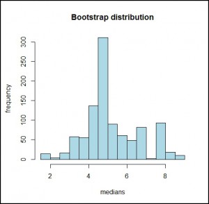
We’re almost there. With all these estimators we construct its distribution which we call bootstrap distribution, which represents an approximation of the true distribution of the statistic in the population. Obviously, this requires that the original sample from which we start is representative of the population. The more different from the population, the less reliable the approximation of the distribution we’ve calculated.

Finally, using the bootstrap distribution we can calculate its central value (the point estimator) and its confidence interval in a similar way as we did for calculating the mean’s confidence interval with the sampling distribution.

Let’s see an example

As you can see, a very nimble procedure that nobody would dare to implement without the help of a statistical program and a good computer. Let’s see a practical example for better understanding.

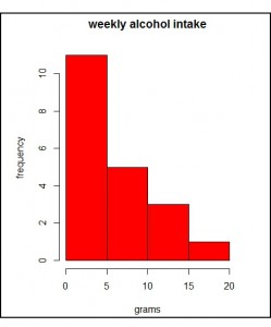
Let’s suppose for a moment that we want to know what the intake of alcohol in a certain group of people is. We collected 20 individuals and calculate their weekly alcohol consumption in grams, with the following results:

You can see the data plotted in the first histogram. As you see, the distribution is asymmetric with a positive bias (to the right). We have a dominant group of teetotalers and scarce drinkers with a tail that represents to those who are taking increasingly higher intakes, which are becoming less frequent. This type of distribution is very common in biology.

In this case the mean would not be a good measure of central tendency, so we prefer to calculate the median. To do this, we can sort the values from lowest to highest and make the average of those in the tenth and eleventh places. I’ve bothered to do it and I know that the median equals (4.77 + 5) / 2 = 4.88.

But now, I’m interested in knowing the value of the median in the population from which the sample comes. The problem is that with such a small and biased sample I cannot apply the usual procedures and I’m not able to collect more individuals from the population to perform the calculation using them. Here’s when bootstrapping comes in handy.

So I obta in 1000 samples with replacement from my original sample and calculate the medians of the 1000 samples. The bootstrap distribution of these 1000 medians is represented in the second histogram. As can be seen, it looks like a normal distribution whose mean is 4.88 and whose standard deviation is 1.43.

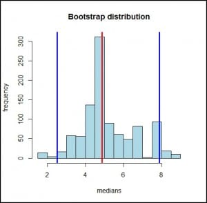
Well, we can now calculate our confidence interval for the population estimate. We can do this in two ways. First, calculating the margins which cover 95% of the bootstrap distribution (calculating the 2.5th and the 97.5th percentiles), as you can see represented in the third graph. I used the program R, but it can be done manually using formulas to calculate percentiles (although it’s not highly recommended, as there are 1000 medians to deal with). So, I get a mean of 4.88 with a 95% confidence interval from 2.51 to 7.9.

The other way is using the central limit theorem that we cannot use with the sampling distribution but can use wi th the bootstrap distribution. We know that the 95% confidence interval is equal to the median plus and minus 1.96 times the standard error (which is the standard deviation of the bootstrap distribution). Then:

95% CI = 4,88 ± 1,96 x 1,43 = 2,08 a 7,68.

As you see, it looks pretty similar to that obtained with the percentile’s approximation.

We’re leaving…

And here we leave the matter for today, before any head overheats in excess. To encourage you a little, all this crap can be avoided resorting to a software like R, which calculates the interval and makes the bootstrapping if necessary, with such a simple command as ci.median() from the asbio library.

This is all for today. Just saying that bootstrapping is perhaps the most famous of the resampling techniques, but it’s not alone. There’re more, some with peculiar names such as jackknife, randomization and validation test or cross-validation test. But that’s another story…