Residuals.

The calculation of the residuals of a contingency table is shown, using the observed and expected values.

We live in a nearly subsistence economy. We do not throw anything away. Even if there’s no choice but to waste something, it is rather recycled. Yes, recycling is a good practice, with its ecological and economic advantages. And the thing is that residues are always usable.

But when it comes to statistics and epidemiology, not only residues are not thrown, they are important for interpreting the data from which they come. Does anyone not believe it?. Let’s imagine and absurd but very illustrative example.

Residuals

Suppose we want to know what kind of fish is the most preferred in Mediterranean Europe. The reason for wanting to know this must be so stupid that it has not yet occurred to me but, anyway, I do a survey among 5,281 people from four countries in Southern Europe.

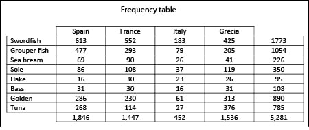
The simpler and most useful thing to do in the first place is the one that is often done always: to build a contingency table with the frequencies of the results, such as I show you below.

Contingency tables

Contingency tables are often used to study the association or relationship between two qualitative variables. In our example, both variables are the preferred fish and the place of residence. Normally, you try to explain a variable (dependent) as a function of the other one (independent). In our example we want to know if the respondent’s nationality influences his or her food tastes.

Total values table is informative in itself. For instance, we see that grouper fish and swordfish are preferred over hake, that Italians like tuna less than Spanish, etc. However, managing large tables like ours can be laborious and difficult to draw many conclusions from raw data. Therefore, a useful alternative is to build a table with percentages of rows, columns or both, as you can see below.

Percentage table

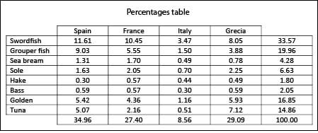
It comes in handy to compare columns’ percentages to check the effect of the independent variable (nationality, in our example) over the dependent variable (preferred fish). Moreover, row’s percentages show the frequency distribution of the dependent variables for each of the categories of the independent one (the country, in our set). But, of the two percentages, the most interesting  ones are column’s percentages: if we see clear differences among categories of the independent variable (countries) we´ll suspect that there may be a statistical association between variables.

In our survey, the percentages within each column are very different, so we suspect that not all fishes are preferred in all countries equally. Of course, this must be quantified in an objective way in order to be sure that these results are no due to chance. How?. Using residuals (the way residues are called in statistics). We’re going to see what they are and how to get them in a while.

Expected values

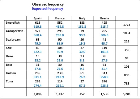
The first thing to do is to build a table with the expected values if all people like all fishes equally, no matter their country of origin. We need to do that because many statistical association and significance tests are based on the comparison between observed and expected frequencies. To calculate the expected value of each cell as if there were not relationship between variables, you have to multiply the row marginal (the row total) by the column marginal and divide them by the total of the table. So, we obtain the table with expected and observed values that I show you below.

If variables are unrelated, observed and expected values are virtually the same, with small differences due to sampling error. If there’re large differences, there will be a likely relationship between the two variables that explains them. And when it comes time to assess these differences is when our residuals come into play.

Residuals

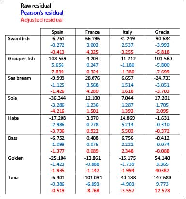
A residual is just the difference between expected and observed values. We already said that when residuals move away from zero they may be significant but, how much do they have to move away?.

We can transform a residual dividing it by the square root of the expected value. So, we come up with the standardized residual, also called Pearson’s residual. In turn, a Pearson’s residual can be divided by the standard deviation of all residuals (square root[(Expected(1-RowProportion)(1-ColumnProportion))]), thus obtaining the adjusted residual. We can now build the residuals table shown below.

The great usefulness of adjusted residuals is that they are standardized values, so we are allowed to compare residuals from different cells. Furthermore, adjusted residuals follow a standard normal frequency distribution (with mean zero and standard deviation one), so we can use a computer program or a probabilities table to come up with the probability that a certain residual’s value is not due to chance. In a normal distribution, 95% of the values are roughly within the mean plus or minus two standard deviations. So, if the adjusted residual’s value is greater than two o lesser than minus two, the probability that this value is due to chance will be less than 5% and we’ll be able to say that the residual is significant. For example, in our table we see that French people like sea bream more than what would be expected if the country did not influence food taste, while, at the same time, they abhor tuna.

Adjusted residuals allow us to assess the significance in each cell but, if we want to know if there’s a global association between variables we have to sum up all adjusted residuals. This is because the sum of adjusted residuals also follow a frequency distribution, but this time it’s a chi-square frequency distribution with (rows-1) x (columns-1) degrees of freedom. If we calculate our value we’ll come up with a chi-square = 368.3921 with a p value <0.001, so we’ll conclude that there’s a statistically significant relationship between the two variables.

We’re leaving…

As you see, residuals are very useful, not only to calculate chi-square, but also to calculate many other statistics. However, epidemiologists prefer to use other measures of association with contingency tables. And this is because chi-square doesn’t vary from zero to one and, although it informs us if there’s statistical significance, gives no information about the strength of the association. For that we need other parameters that do vary from zero to one, such us the risk ratio and the odds ratio. But that’s another story…